What the paper contributes
Qiyuan Wang, Ke Xiao and Christos Anagnostopoulos posted Discount Yourself on 20 October 2026. Their SFG-L rule weights every candidate, including the receiver, using inherited lag. The paper bounds aggregation error; it does not prove convergence of training. Its synchronous image-classification experiments also leave deployment questions open. Original paper and full text, especially Sections 4–7 and Appendix A.2.
The calculations and research questions below are an independent reading aid. They are not reproduced experiments.
A comic you can check
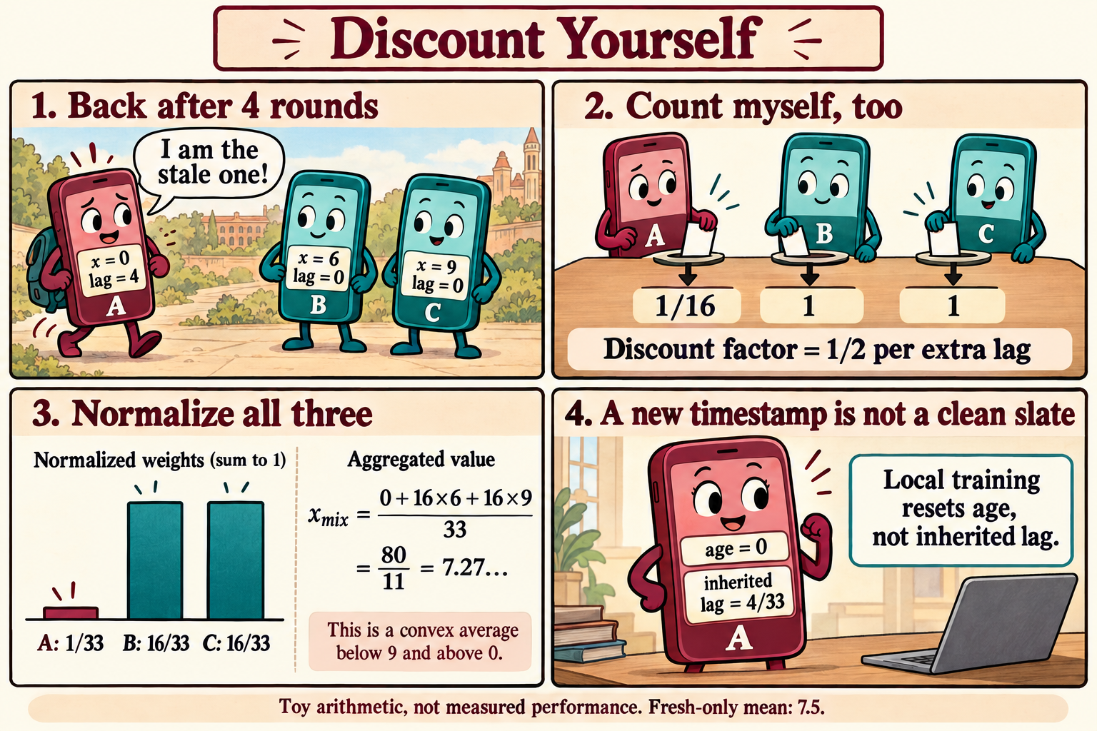
Read left to right, then down. A returns after four missed rounds. With a discount of one half per extra lag, its raw vote is 1/16; the other votes are 1 each. Normalizing gives 1/33, 16/33, 16/33. The fourth panel tracks inherited lag after mixing and local training, without another outage. All numbers are illustrative.
Original calculation: when should self-weight fall?
Imagine three phones exchanging models without a central server. One phone has just returned after four rounds offline. Its neighbours have continued learning. Model ownership gives no mathematical reason to trust it more; its information matters.
Let the current target be c, the returning model be x₀, and the fresh models be x₁,x₂. For this toy calculation, assume independent, zero-mean errors. Each fresh model has variance σ²; the old model has variance σ² + τδ², representing τ missed independent drift increments. This independence assumption simplifies the calculation and is not a claim about arbitrary gossip networks.
Give the old model weight a, and each fresh model weight (1−a)/2. Its expected squared error is
\[R(a)=a^2(\sigma^2+\tau\delta^2) +\frac{(1-a)^2}{2}\sigma^2.\]The first term penalizes trusting the old model; the second rewards averaging independent fresh estimates. Differentiating,
\[R'(a)=2a(\sigma^2+\tau\delta^2)-(1-a)\sigma^2, \qquad R''(a)=3\sigma^2+2\tau\delta^2>0.\]Thus, for positive σ² and nonnegative τ,δ², the unique minimum is
\[a^\star=\frac{1}{3+2\tau\rho}, \qquad \rho=\frac{\delta^2}{\sigma^2}.\]With no missed progress, the optimal self-weight is one third. As the outage grows, it falls. Equal treatment is justified by equal uncertainty, rather than by the presence of three devices.
Set σ² = δ² = 1 and τ = 4. Then
\[R(a)=5a^2+\frac{(1-a)^2}{2}.\]Uniform averaging has risk 7/9; the one-step optimum uses a = 1/11 and has risk 5/11. These are exact toy-model calculations.
The paper’s rule, applied to our numbers
SFG-L uses geometric weights:
\[w_j=\frac{\gamma^{\ell_j-\ell_{\min}}} {\sum_{k\in S}\gamma^{\ell_k-\ell_{\min}}}, \qquad \ell_{\min}=\min_{k\in S}\ell_k.\]S includes the receiver; ℓⱼ is effective lag and 0 < γ < 1. See Equation (8) and the lag-based instantiation in Section 5.
For γ = 1/2 and lags (4,0,0), the raw weights are (1/16,1,1). Their sum is 33/16, so
\[(w_0,w_1,w_2)=\left(\frac1{33},\frac{16}{33},\frac{16}{33}\right).\]For scalar model values (0,6,9),
\[x_{\mathrm{mix}}=\frac{0+16\cdot6+16\cdot9}{33} =\frac{80}{11}\approx7.27.\]Uniform averaging gives 5; averaging only the fresh models gives 7.5. This establishes the arithmetic, not that 7.27 is the correct target.
Under our variance assumptions, the geometric rule has risk 47/99, slightly above the one-step optimum 5/11. A convenient freshness rule need not be optimal for every estimation problem. Its value needs assessment across the learning process.
Under the paper’s bookkeeping, effective lag is a weighted inheritance when available, or an increment when offline:
\[\ell_i^+=\sum_{j\in S}w_j\ell_j \quad\text{(available)},\qquad \ell_i^+=\ell_i+1 \quad\text{(offline)}.\]Our returning phone inherits lag 4/33, rather than zero. Local training can reset its age without erasing inherited lag. See Equation (21).
Original analysis: freshness can change influence
For optimization research, a further question is which objective the network actually optimizes. Consider this independently chosen mixing matrix:
\[W=\begin{pmatrix}0.1&0.9\\0.2&0.8\end{pmatrix}, \qquad W\begin{pmatrix}0\\10\end{pmatrix} =\begin{pmatrix}9\\8\end{pmatrix}.\]Every row sums to one: each client forms a valid convex combination. Yet the network mean moves from 5 to 8.5. Convex combinations preserve a constant model without necessarily preserving the average model. This example is an algebraic caution, not a counterexample to the paper’s stated aggregation-error results.
In infrastructureless learning, I would investigate freshness and representation together. Frequently connected clients may offer recent progress while representing a narrow population. Reducing temporal error might increase population bias; these effects need separate measurements.
A useful first experiment would fix graph, data partitions, initial models and outage traces. Compare uniform mixing, age weighting and inherited-lag weighting. Measure recovery after reconnection, average accuracy, low-availability clients and the effective contribution of each population. First make outages independent of labels, then deliberately couple them.
For random-walk ADMM, replacing an averaging coefficient requires further care: primal variables, dual variables and local objective weights play different roles. I would begin with convex quadratic objectives, whose intended solution can be calculated exactly, and check whether the adaptive weights shift it.
The next theoretical question is specific: under which conditions do freshness weights preserve the intended solution while controlling missed-progress errors? An old model can deserve less weight while its owner’s data still deserves the influence promised by the learning objective.
Sources and reading boundary
- Paper metadata and version date.
- Full text: model assumptions in Sections 4.1 and 4.3; weighting and lag updates in Equations (8), (20)–(21); limitations in Section 7 and Appendix A.2.
- PDF.
Read on 24 October 2026. Prepared with Codex; mathematical comic generated with ImageGen and checked against the worked example. No training experiments were run for this note.