When Softmax Loses a Small Gradient

The paper and the question

Jonathan T. Barron, Dan Gnanapragasam and Michael Tschannen posted A Fix for Softmax and Cross-Entropy on 22 October 2026. They study numerical failures in high-confidence classification and near-matching teacher/student predictions, and propose stable reformulations. Their evaluation covers arithmetic-learning and distillation settings; it does not establish universal training acceleration. The margin-equilibrium discussion uses approximate assumptions about optimizer moments and gradient decay. Full text, Sections 2–7.

This note focuses on the hard-target case in Section 2. The worked arithmetic, invariance argument and proposed diagnostics below are an independent explanation. We verified scalar rounding operations, not a training run or a framework implementation.

Four panels, one rounding error

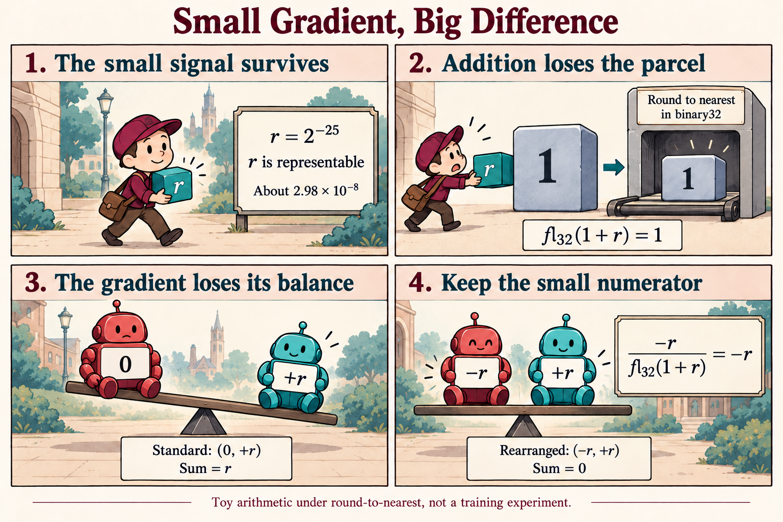
The parcel r is an already-computed, exactly representable residual. Under round-to-nearest binary32 arithmetic, adding it to one loses it. The standard target gradient becomes zero while the other gradient stays positive. Keeping the small numerator restores opposite gradient entries in this toy example.

Start with a mathematical invariant

Let z be a vector of K finite logits, t the target class, and L the hard-target cross-entropy. In exact arithmetic,

Adding the same scalar c to every logit cannot change this loss:

Differentiating with respect to c at zero gives

This is a useful implementation check. The gradient should have no component along the common-shift direction. It describes sensitivity to the logits, rather than to every parameter of the network.

For two classes, let m be the target logit’s margin over the other logit and set r equal to exp(-m). Then

The two target-gradient expressions are algebraically equal. Their operation sequences can lose different information. This is the key contrast in Section 2, Equation (3).

An original binary32 calculation

Choose the residual directly:

We start after exponentiation so that the rounding effect is isolated. We do not assume a binary32 logit can represent the corresponding irrational margin, 25 log(2), exactly.

Assume IEEE binary32 and round to nearest. The next representable number above one is 1 + 2 to the power -23; the midpoint is 1 + 2 to the power -24. Our r is smaller than the midpoint distance. Therefore,

The standard operation sequence computes

Its gradient sum is r. A small signal has disappeared from only one entry.

Rearrange the target expression before evaluating it:

Now the computed sum is zero. The exact real-valued target gradient remains -r/(1+r); the computed value -r is a floating-point approximation, not a claim of exact real arithmetic.

The forward loss has a related issue: log(d) is zero, while a stable log1p(r) calculation preserves approximately r. A short verification rounds each operation explicitly:

import math
import struct

def f32(x):
    return struct.unpack("<f", struct.pack("<f", x))[0]

r = f32(2.0 ** -25)
d = f32(f32(1.0) + r)
other = f32(r / d)
standard = (f32(f32(1.0 / d) - 1.0), other)
rearranged = (f32(-r / d), other)

assert d == 1.0 and standard[0] == 0.0
assert f32(sum(standard)) == r
assert f32(sum(rearranged)) == 0.0
assert f32(math.log1p(r)) == r

This verifies the stated operation sequence. It does not model every fused kernel, reduction order or autodifferentiation rule. Python’s log1p call is evaluated in binary64 before the result is rounded to binary32.

Original analysis: zero-sum is necessary, not sufficient

It is tempting to repair a bad gradient by projecting it onto the zero-sum subspace. For two classes the Euclidean projection is

The sum is now zero, but both entries have roughly half the correct magnitude. Relative to the rearranged vector (-r,r), its Euclidean error is 50 percent. Passing an invariant check cannot establish that the useful gradient signal was recovered.

This suggests two complementary diagnostics for an optimization pipeline. First, check structure: the sum over logit gradients, invariance to a common logit shift, and the expected sign on the target. Second, check magnitude against a higher-precision reference across margins. A tiny absolute error can hide a large relative error when the true gradient itself is tiny.

I would begin with deterministic logits before comparing training curves. Sweep margins through the precision boundary, vary the number of classes, and inspect the actual backward path. Test the deployed kernel and dtype, rather than inferring behavior from a mathematically stable forward formula alone.

For efficient training or model adaptation, this gives a useful attribution question. If an apparent optimizer failure changes when only the loss arithmetic changes, part of the effect belongs to the numerical objective implementation. Label smoothing, soft targets and distributed reductions introduce additional questions; our binary hard-target calculation does not settle them.

What to carry into research

The paper’s broader fix constructs a stable loss through target-relative differences and an appropriate softplus operation; its autodiff path matters. See Section 2, Equations (6)–(7). The one-line rearrangement in our toy is an explanation, not a complete multiclass loss implementation.

A concrete next experiment is to hold initialization, batches, optimizer and learning-rate schedule fixed while changing only the cross-entropy implementation. Record gradient-reference error alongside loss and accuracy. That would distinguish a numerical correction from a change in statistical learning behavior.

The lesson is operational: preserve the small quantity before subtraction destroys it, and verify both the gradient’s structure and its scale.

Sources and verification

• Version and authors, first posted 22 October 2026.
• Full text: hard-target reformulation in Section 2; separate soft-target treatment in Section 3; approximate equilibrium analysis in Section 5; evaluations in Sections 6–7.
• PDF.

Read on 25 October 2026. Prepared with Codex. The four-panel comic was generated with ImageGen and corrected after checking its arithmetic labels. No training or framework benchmark was reproduced for this note.