The paper and the question
Haodong Wen and colleagues posted Data Schedules and Learning Rate Schedules Should Be Designed Together on 21 October 2026. They study pretraining (PT) and target mid-training (MT) allocations under fixed compute and MT-data budgets. Their experiments show that changing the learning-rate schedule can reverse data-schedule rankings. Their theory uses noisy quadratic objectives and an SDE approximation. Original paper, Sections 2–3.
A finite, two-step stochastic model makes this interaction visible through exact expected losses.
Four panels, one ranking reversal
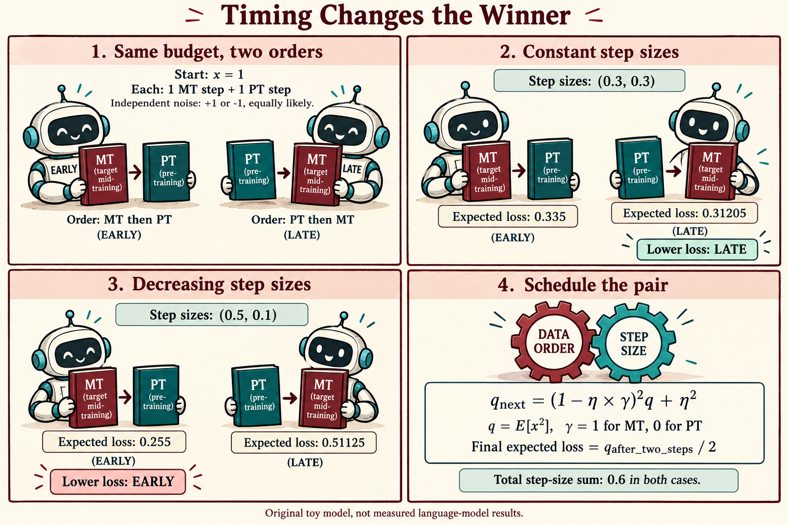
EARLY uses MT then PT; LATE uses PT then MT. Both use one step of each kind. Each learning-rate profile sums to 0.6. The winning order changes when those step sizes are redistributed.
Define the noisy oracle
Consider one target coordinate x, starting at one. Define
\[f_{\mathrm{PT}}(x)=0,\qquad f_{\mathrm{MT}}(x)=\frac{x^2}{2},\qquad x_0=1.\]PT is deliberately flat along this coordinate. It can represent a direction relevant to the target task but absent from the pretraining objective. We nevertheless give both kinds of oracle the same noise. This is an explicit modeling choice, not a claim about pretraining data generally.
At each step t, let gamma be one for MT and zero for PT. The oracle and update are
\[g_t=\gamma_t x_t+\xi_t,\qquad x_{t+1}=(1-\eta_t\gamma_t)x_t-\eta_t\xi_t.\]The noises are independent, each equally likely to be +1 or -1, and independent of the past. Step sizes and data order are fixed in advance. Therefore the oracle is unbiased conditional on the current state, and its noise variance is one.
The comparison gives each procedure exactly two equally costly oracle calls: one MT and one PT. This call budget is an illustrative analogue of a data budget, without claiming that one oracle call describes a language-model batch.
Derive the expected loss
Let q be the second moment of the target coordinate. Squaring the update produces a cross term whose expectation vanishes because the new noise has conditional mean zero:
\[q_{t+1} =(1-\eta_t\gamma_t)^2q_t+\eta_t^2, \qquad q_0=1.\]The final expected target loss is q after two steps divided by two. Write the first step size as a and the second as b.
For EARLY, the MT step contracts the initial coordinate and the following PT step adds noise:
\[q_1=(1-a)^2+a^2,\qquad R_{\mathrm{E}}=\frac{(1-a)^2+a^2+b^2}{2}.\]For LATE, the first PT step adds noise, which the final MT step partly contracts:
\[q_1=1+a^2,\qquad R_{\mathrm{L}}=\frac{(1-b)^2(1+a^2)+b^2}{2}.\]These equations retain both the squared mean and the noise variance. Following only the mean trajectory would miss the advantage of a late contracting step under constant learning rates.
Equal budgets, different winners
Compare a constant profile (0.3, 0.3) with a decreasing profile (0.5, 0.1). Both have total step-size sum 0.6. Within each profile, the orders also share the same per-step learning rates.
| Step-size profile | EARLY: MT then PT | LATE: PT then MT |
|---|---|---|
| Constant (0.3, 0.3) | 0.335 | 0.31205 |
| Decreasing (0.5, 0.1) | 0.255 | 0.51125 |
Bold values mark the lower expected loss in each row.
For the constant profile, both final means are 0.7. EARLY has variance 0.18; LATE has variance 0.1341 because the final MT step attenuates the first noise contribution. Their difference is entirely variance.
More generally, setting both step sizes to c gives
\[R_{\mathrm{E}}-R_{\mathrm{L}} =\frac{c^2}{2}\left[1-(1-c)^2\right] =\frac{c^3(2-c)}{2}>0 \quad\text{for }0<c<2.\]Thus LATE wins throughout the contractive constant-step range in this toy.
With decreasing steps, EARLY applies the target gradient at step size 0.5, leaving a final mean of 0.5. LATE applies it at 0.1, leaving a mean of 0.9. EARLY’s squared mean and variance are 0.25 and 0.26; LATE’s are 0.81 and 0.2125. The stronger early reduction of the mean outweighs its larger variance.
The target-call count stays fixed, but the target-gradient exposure depends on where that call lands:
\[\sum_t\gamma_t=1,\qquad \sum_t\eta_t\gamma_t= \begin{cases} a,&\text{EARLY},\\ b,&\text{LATE}. \end{cases}\]Raw data counts leave this optimizer-weighted exposure uncontrolled. That is precisely why order and step size make a joint choice.
Account for every noise path
There are only four equally likely noise pairs. This exact-fraction enumeration checks the second-moment derivation without Monte Carlo error:
from fractions import Fraction as F
from itertools import product

def expected_loss(step_sizes, order):
    total = F(0)
    for noises in product((-1, 1), repeat=2):
        x = F(1)
        for eta, gamma, noise in zip(step_sizes, order, noises):
            x = (1 - eta * gamma) * x - eta * noise
        total += x * x / 2
    return total / 4

early, late = (1, 0), (0, 1)
constant = (F(3, 10), F(3, 10))
decreasing = (F(1, 2), F(1, 10))

assert sum(constant) == sum(decreasing) == F(3, 5)
assert expected_loss(constant, early) == F(67, 200)
assert expected_loss(constant, late) == F(6241, 20000)
assert expected_loss(decreasing, early) == F(51, 200)
assert expected_loss(decreasing, late) == F(409, 800)
This finite noisy-oracle example is not a proof of the paper’s continuous-time results, nor evidence that early target data always wins with decay.
Read the theory with its conditions
The paper’s constant-rate and reversal results have formal conditions in Appendices I–K. Its explicit three-stage optimum additionally uses a spectral/noise model and a sufficiently long horizon; the delayed-decay result has further budget and spectral restrictions. The paper leaves general joint optimization and broader training objectives open.
Our example assumes a deterministic schedule, equal call costs, flat PT curvature in the target coordinate, independent additive noise and a quadratic MT objective. Correlated noise or a useful PT gradient in that coordinate would change the calculation. Matching the sum of learning rates also leaves their squared sum different, affecting injected noise; the comparison specifies that difference rather than hiding it.
A useful experiment for adaptation research
For a foundation-model adaptation experiment, I would cross each candidate data schedule with several learning-rate profiles before attributing gains to the curriculum. Keep initialization, total compute, source-wise token counts, batch construction and evaluation fixed. Report the pair of schedules, where target data first enters, and the resulting optimizer-weighted target exposure.
Repeated seeds would be needed for empirical uncertainty. A loss improvement on the target distribution should also be checked alongside the retained pretraining distribution and the downstream task. Our scalar example optimizes only the final target quadratic and provides no retention guarantee.
For federated learning, a related research question is whether a client-sampling curriculum retains its apparent benefit when crossed with step-size schedules. Heterogeneity, client availability and communication costs would need their own model; the toy calculation supplies a diagnostic question, not a federated convergence result.
Treat the data schedule and the learning-rate schedule as a single experimental choice.
Sources
- Authors, first-publication date and version.
- Full text: Section 3 and Appendix H define the noisy quadratic setup; Appendix J develops its bias/variance analysis; Appendices I–K and N state the theorem conditions and proofs.
- PDF.
The comic was created with AI.