The paper and the question
Junyu Lin and colleagues posted FedGRC on 22 October 2026. It combines shared representation learning, a covariance metric and class-mean personalization. Evaluation includes classes absent from each client’s training set but known elsewhere in the federation. Full paper, Sections III–V.
A class can retain its shared mean while losing predictions to a moving competitor. The following original example makes that distinction concrete.
Four panels, one moving boundary
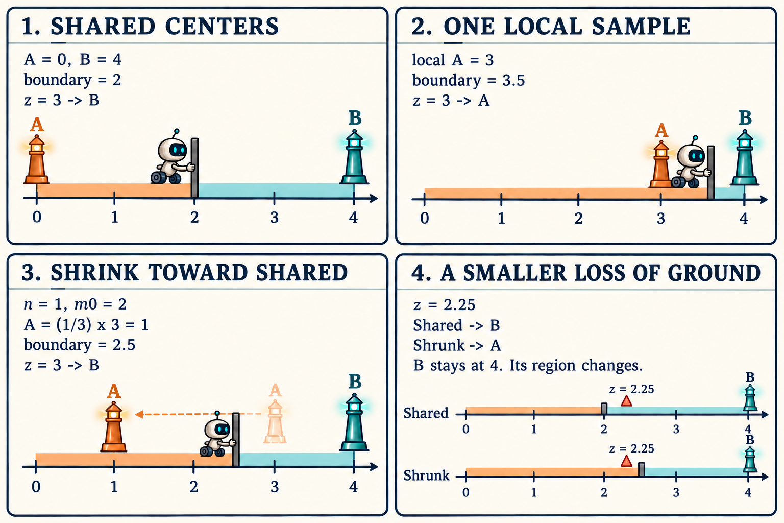
Class B stays at 4 throughout. Direct local adaptation moves the boundary from 2 to 3.5. Shrinkage pulls it back to 2.5, restoring the B prediction at 3 while still changing the prediction at 2.25.
Why the average needs a second view
Imagine a client whose test distribution contains 99% class A and 1% class B. A predictor that always selects A has 99% local accuracy but only 50% accuracy under equal class frequencies. Those scores describe the same predictor under different distributions.
That arithmetic alone says nothing about which deployment distribution matters. It does show why a local average cannot answer a class-coverage question. In a medical or remote-sensing federation, an infrequent category can remain scientifically important even when it barely changes the average.
Define the personalization rule
For one class, let b be its shared center, let n local features be z_i, and let lambda be a positive reference strength. With a fixed positive-definite metric M, FedGRC’s mean-fitting objective gives
\[J(m)=\sum_{i=1}^{n}\|z_i-m\|_M^2 +\lambda\|m-b\|_M^2, \qquad m^\star=\frac{\sum_i z_i+\lambda b}{n+\lambda}.\]Here the squared metric norm is v-transpose M v. The local mean receives weight n/(n+lambda); an empty local sample leaves b unchanged. This is Proposition IV.2 and Appendix A-F, with lambda denoting the paper’s m_0. Derivation in the source.
Our example fixes the scalar metric to one and uses equal class priors. Both centers are supplied as fixed shared statistics: A at zero and B at four. The client has one A feature at three and no B examples. The reference strength is two, chosen for this example.
The A objective and its derivatives are simply
\[J_A(m)=(3-m)^2+2m^2,\qquad J_A'(m)=6m-6,\qquad J_A''(m)=6.\]Thus its unique minimizer is one. Equivalently, the local weight is 1/(1+2)=1/3, so the shift from zero to three is reduced to one. For B, the objective is 2(m-4)^2 and the minimizer remains four.
Shared centers can be compatible with these local data: for instance, two A features of -1.5 elsewhere would balance this client’s feature of three to a federation-wide mean of zero. We are isolating the final classification geometry, without changing features or fitting a covariance from this tiny sample.
Compare three classifiers
Use the nearest-center decision rule. When the A center is a and the B center is four, compare their squared distances:
\[(z-4)^2<(z-a)^2 \quad\Longleftrightarrow\quad 2(4-a)z>16-a^2.\]For a below four, B therefore wins when z exceeds (a+4)/2. All points below are away from ties.
| Classifier | A center | Boundary |
|---|---|---|
| Shared | 0 | 2 |
| Direct local | 3 | 3.5 |
| Shrunk | 1 | 2.5 |
The B center is four in every row. For a query at three labeled B, the shared classifier predicts B. Direct adaptation predicts A because that query now sits exactly at the A center. Shrinkage restores B: its distances to A and B are two and one.
Now consider another B-labeled query at 2.25. Its shared distances are 2.25 to A and 1.75 to B, so the shared classifier is correct. After shrinkage, the distances are 1.25 to A and 1.75 to B: the prediction becomes A.
These are pointwise examples. They do not specify a population or establish an accuracy ranking.
Derive the region that changes
Let a local A center move from zero to a positive value d below four. A shrinkage weight alpha between zero and one produces the adapted center alpha d. The boundary becomes
\[t_\alpha=2+\frac{\alpha d}{2}.\]Relative to the shared classifier, B loses the open interval from 2 to this new threshold. Its width is alpha d/2, compared with d/2 under direct adaptation. Shrinkage reduces this width linearly, but a positive displacement leaves a nonempty interval.
For d=3, the direct loss of ground has width 1.5. With alpha=1/3 it is 0.5. The query at three lies in the recovered portion; the query at 2.25 lies in the portion still lost.
Preserving B at 2.25 requires a stricter choice:
\[2+\frac{3\alpha}{2}<\frac94 \quad\Longleftrightarrow\quad \alpha<\frac16.\]With one local sample, alpha=1/(1+lambda), so lambda must exceed five. Equality puts this query on the decision boundary and depends on tie-breaking.
A stronger shared reference can preserve this particular B prediction, while also limiting adaptation to a real A-specific shift. Class support alone does not decide that tradeoff: the displacement and the queries’ margins matter too.
An exact arithmetic example
The linear score mu*z-mu^2/2 differs from negative one-half squared distance by a term common to both classes. It gives the same decisions. This short calculation makes the competing scores explicit:
from fractions import Fraction as F

def score(z, mu):
    return mu * z - mu * mu / 2

def predict(z, a):
    sa, sb = score(z, a), score(z, F(4))
    assert sa != sb
    return "A" if sa > sb else "B"

centers = (F(0), F(3), F(1))
assert [predict(F(3), a) for a in centers] == ["B", "A", "B"]
assert [predict(F(9, 4), a) for a in centers] == ["B", "A", "A"]
assert [(a + 4) / 2 for a in centers] == [F(2), F(7, 2), F(5, 2)]

# B's score stays fixed while A's score changes.
assert score(F(9, 4), F(4)) == 1
assert score(F(9, 4), F(1)) == F(7, 4)
What the proof establishes
The paper’s stability result is conditional on fixed fitted statistics: a shared winning margin larger than the combined score-perturbation bound preserves that prediction. It establishes neither correctness of the shared prediction nor universal improvement from adaptation. Corollary IV.1 and Appendix A-H.
Our scalar result is sharper for this specific configuration because it solves the boundary exactly. It does not analyze learning the representation, uncertainty in the shared means, unequal priors, multiple competing classes, or a changing metric. The chosen reference strength is illustrative rather than a tuned operating point.
A useful test for federated personalization
I would evaluate a personalization rule by tracking changed decisions, in addition to unchanged class statistics. Freeze the backbone and metric first, vary the reference strength, and compare shared and personalized predictions on held-out examples. Record class support, center displacement and the shared margin for every flip.
Separate correct-to-incorrect flips from incorrect-to-correct flips, and report them for locally absent, sparsely observed and well-observed classes. A small aggregate change could hide a large exchange between those groups. Then repeat with learned representations and several client partitions to see which behavior survives beyond the fixed geometry.
This also suggests a research direction: select adaptation strength using both support and a constraint on damaging boundary movement. The constraint would need held-out evidence and uncertainty estimates; preserving every shared decision would also prevent beneficial corrections. A useful design should expose that exchange rather than assume a fixed mean protects a class.
Sources
- Lin, Qi, Shi and Li, Is High Local Accuracy Enough? Geometric Consensus with Support-Adaptive Statistical Personalization for Federated Learning, v1, first posted 22 October 2026.
- Complete text and proofs: Section IV-C; Appendices A-F and A-H.
- PDF.
The comic was created with AI.