The paper and the question
Zhirayr Tovmasyan and colleagues posted SCAFFOLD under Hessian Similarity: Sharp Convergence Rates on 26 October 2026. Their convex analysis connects the benefit of local computation to similarity of client curvature. Full paper, Sections 2–3.
A useful question for federated optimization is whether checking each client’s step size is enough. The original example below gives a precise answer for the paper’s update: two contracting local maps can form an unstable server recurrence.
Four panels, two kinds of stability
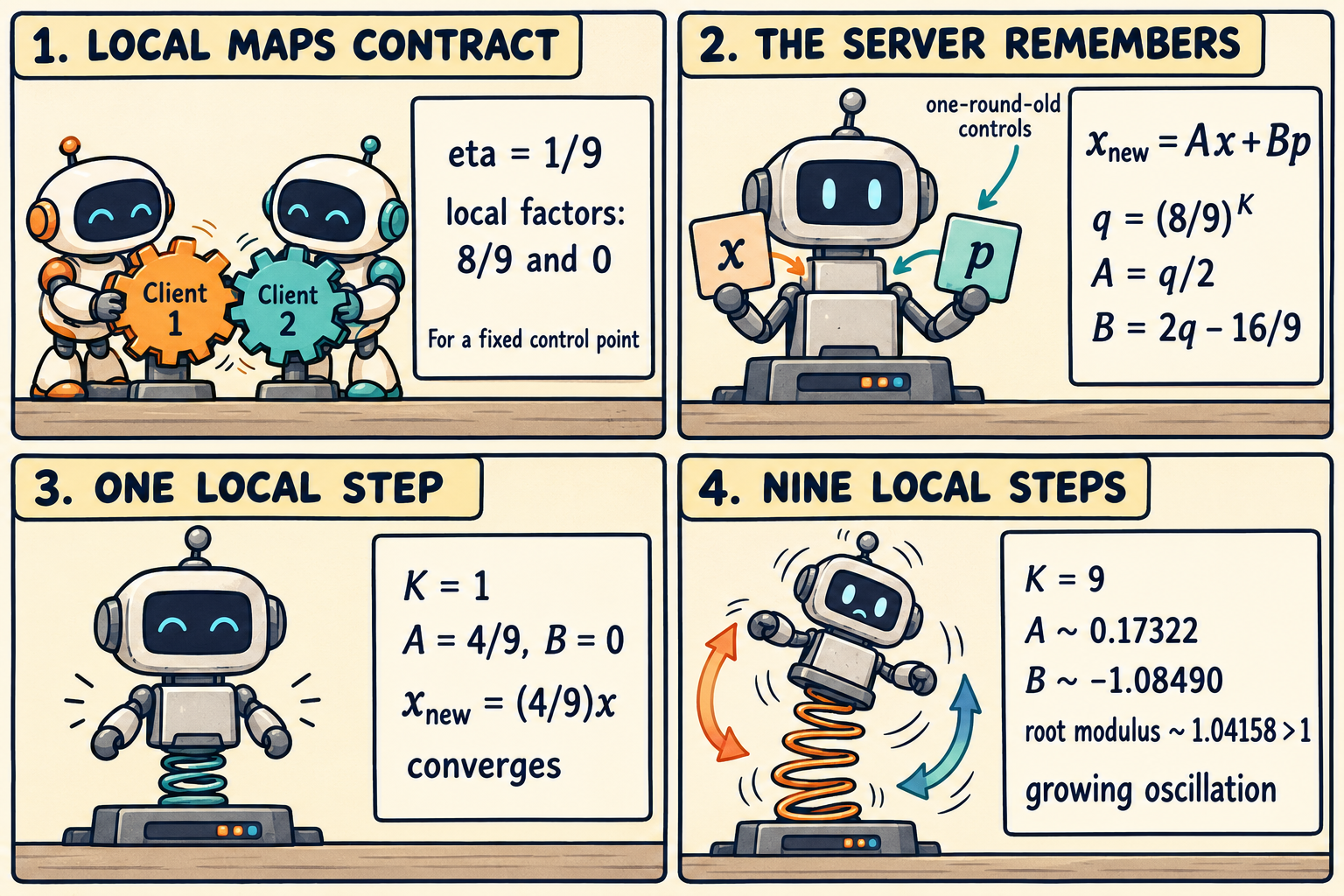
The local factors stay at 8/9 and zero. Increasing the number of local steps changes how strongly the server depends on the previous control point. At nine steps, the server oscillation has a growing envelope.
Two convex clients
Consider scalar objectives
\[f_1(x)=\frac{x^2}{2}+10x,\qquad f_2(x)=\frac{9x^2}{2}-10x.\]Their equally weighted global objective is f(x)=5x^2/2, with minimizer zero. Both clients participate in every round. All gradients are exact, the server averages the two endpoints, and the local step size stays at eta=1/9.
The local curvatures are one and nine, so their common smoothness bound is L_loc=9. The global curvature is five. The root-mean-square deviation of local curvatures from five is
\[\delta=\sqrt{\frac{(1-5)^2+(9-5)^2}{2}}=4.\]The affine offsets of +10 and -10 create large gradient disagreement but do not change curvature. They will cancel from the corrected updates.
Keep the control timing explicit
Algorithm 1 uses controls evaluated one server iterate before the local starting model, with x^(-1)=x^0 at initialization. This is its minibatch Option-I timing, rather than a same-round refresh. Algorithm 1 and Equation (10).
Write the current starting model as x and the older control point as p. For our deterministic objectives, the client controls and their average are
\[c_1=p+10,\qquad c_2=9p-10,\qquad c=5p.\]A corrected direction is the client’s gradient minus its control plus the average control. Substitution gives
\[v_1(y)=y+4p,\qquad v_2(y)=9y-4p.\]For a fixed p, the resulting local affine maps have slopes 8/9 and zero. Each is a contraction toward its own fixed point. This statement does not say that either fixed point is the global minimizer.
At a common evaluation point y, the corrected directions differ from the global gradient 5y by -4(y-p) and +4(y-p). Curvature mismatch therefore reappears as the iterate moves away from the control point.
Only when x=p do both clients start with the same direction 5x. That is true in the first round under the prescribed initialization; later rounds generally start with x different from p.
Solve a complete communication round
Let K be the positive number of local steps and set q=(8/9)^K. Starting both clients at x, their step recurrences are
\[y_{1,k+1}=\frac89y_{1,k}-\frac49p, \qquad y_{2,k+1}=\frac49p.\]The first is a geometric sum; the second reaches its fixed point immediately. Their endpoints are
\[y_{1,K}=qx-4(1-q)p,\qquad y_{2,K}=\frac49p.\]Averaging the endpoints gives the exact server recurrence
\[x^r=A_Kx^{r-1}+B_Kx^{r-2},\qquad A_K=\frac q2,\qquad B_K=2q-\frac{16}{9}.\]Use x^(-1)=x^0=1. The two-dimensional state is the pair of consecutive server models. Checking a scalar client map leaves this memory state out of the calculation.
One step converges; nine steps oscillate outward
For K=1, q=8/9. Then B_K vanishes and the server reduces to x^r=(4/9)x^(r-1), which converges to zero.
For K=9, the coefficients are approximately
\[q=0.3464394161,\qquad A_9=0.1732197081,\qquad B_9=-1.0848989455.\]The characteristic equation is t^2-A_K t-B_K=0. At K=9 its discriminant is negative, so the roots are a complex-conjugate pair. Their product is -B_9, giving the common modulus
\[|t|=\sqrt{-B_9} =\sqrt{\frac{16}{9}-2\left(\frac89\right)^9} \approx1.041584824>1.\]The nonzero initial state therefore excites a growing oscillation. Its first four server models are approximately -0.91168, -1.24282, 0.77380 and 1.48237. The signs and magnitudes need not change monotonically.
| Local steps | Largest root magnitude | Behavior |
|---|---|---|
| 1 | 0.444444 | Converges |
| 8 | 0.999144 | Slow decay |
| 9 | 1.041585 | Growing envelope |
For this family, the stability threshold can also be obtained exactly. For every positive K, A_K is positive and at most 4/9, while the root product C_K=-B_K is nonnegative. If the roots are real, the nonnegative product and positive sum make both roots nonnegative; each is at most A_K and therefore below one. If they are complex, their modulus is the square root of C_K. Thus strict stability is equivalent to
\[C_K<1 \quad\Longleftrightarrow\quad \left(\frac89\right)^K>\frac7{18}.\]K=8 satisfies this inequality narrowly; K=9 does not. This threshold belongs to the particular objectives and fixed step size chosen here.
Follow the literal client updates
The following exact-fraction calculation refreshes controls only after using the old ones. It compares the resulting endpoints with the derived recurrence.
from fractions import Fraction as F

def run(K, rounds=4):
    x, p = F(1), F(1)
    c1, c2 = x + 10, 9*x - 10
    q = F(8, 9)**K
    A, B = q/2, 2*q - F(16, 9)
    out = []
    for _ in range(rounds):
        c = (c1 + c2)/2
        y1 = y2 = x
        for _ in range(K):
            y1 -= (y1 + 10 - c1 + c)/9
            y2 -= (9*y2 - 10 - c2 + c)/9
        nxt = (y1 + y2)/2
        assert nxt == A*x + B*p
        c1, c2 = x + 10, 9*x - 10
        p, x = x, nxt
        out.append(x)
    return out

assert run(1) == [F(4, 9)**r for r in range(1, 5)]
assert run(9)[0] == F(-353203216, 387420489)
assert F(8, 9)**8 > F(7, 18) > F(8, 9)**9
Nine local steps cost more computation per round than one. This comparison diagnoses stability at a fixed step size; it is not a comparison at equal computation budgets.
Read the convergence conditions together
For convex smooth clients under full participation and averaged Hessian similarity, Proposition 1 requires both
\[\eta L_{\mathrm{loc}}\leq1,\qquad K\eta\delta\leq\frac{1}{3\sqrt2}.\]With suitable steps, the exact-gradient guarantee for the average server model scales as
\[f(\bar x^R)-f^\star =O\!\left(\left(\frac{L_{\mathrm{loc}}}{K}+\delta\right) \frac{D_0^2}{R}\right).\]D_0 is the initial distance to a minimizer. Proposition 1, Equation (15), and Appendix A.
Our eta satisfies the local condition exactly. The round-level quantity is 4K/9, which exceeds 1/(3 sqrt(2)) even at K=1. Both compared settings lie outside that sufficient guarantee. The stable K=1 result follows from our exact recurrence; the K=9 result contradicts no theorem.
The paper measures the objective at the average server model. Our calculation concerns stability of the server iterates themselves. It also assumes scalar quadratics, exact controls, equal client weights, fixed participation and a constant local step. It does not settle stochastic training or other SCAFFOLD control-update variants.
What I would measure in a federated experiment
I would tune the local step size and K jointly, recording both etaL_loc and Keta*delta when reliable curvature information is available. Client disagreement, movement from the control point and server oscillations would be useful diagnostics, but finite measurements should not be treated as uniform bounds over the training domain.
I would compare a fixed local step with a rule that reduces it as K grows, and report communication rounds alongside gradient evaluations, including control estimation. That separates additional computation from a useful communication gain.
The exact recurrence points to a further question: how much local work can a control tolerate before its old anchor dominates the server dynamics? A practical answer could use displacement or curvature diagnostics to trigger synchronization. Such a rule needs its own analysis and cost accounting; local contraction alone supplies no guarantee.
Sources
- Tovmasyan, Hanzely, Shulgin, Richtárik and Stich, SCAFFOLD under Hessian Similarity: Sharp Convergence Rates, v1, first posted 26 October 2026.
- Full text and proofs: Assumptions 1 and 3; Algorithm 1; Proposition 1; Appendix A.
- PDF.
The comic was created with AI.