The paper and the question
Abdelghani Belgaid posted Algorithmic Monoculture in Machine Learning-based Site-Specific Fertilizer Recommendation on 27 October 2026. It studies assigning models across farms, with a penalty on aggregate recommendation error. Full paper.
For precision-agriculture AI, a model leaderboard is only one input to deployment design. The following original example holds every model’s individual error distribution fixed while changing how their errors occur together. The preferred deployment changes.
Four panels, two error worlds
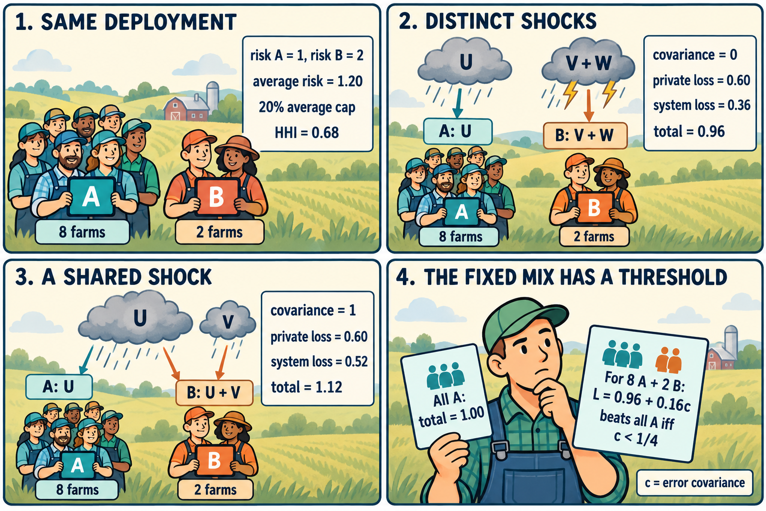
Both worlds use eight A farms and two B farms. Their individual risks, average-risk budget and concentration index agree. The total modeled loss falls from 1.00 to 0.96 in one world and rises to 1.12 in the other.
Define a population loss
Use the paper’s covariance formulation in a scalar example with only model-common errors and a unit systemic penalty. Let q_m be the share assigned to model m, r_m its mean squared error, and Sigma the covariance matrix of the zero-mean model errors. Then
\[L(q)=\underbrace{\frac12\sum_mq_mr_m}_{\text{private term}} +\underbrace{\frac12q^\top\Sigma q}_{\text{system term}}.\]This specializes Equation (4) to rho=1 and lambda=1. Each farm uses one model. Section 3, Equations (4) and (7).
Here a common error means that every farm assigned a model receives the same realized error in that draw. Our construction has no farm-specific error. The loss and all quantities below are dimensionless.
We use ten farms, model A with risk one, and model B with risk two. If x is B’s adoption share, the average squared-error risk is
\[(1-x)\cdot1+x\cdot2=1+x.\]A 20% average-risk cap relative to all A requires x at most 0.2. With ten indivisible farms, the feasible B shares are zero, 0.1 and 0.2. Focus first on eight A farms and two B farms.
Keep the marginal errors identical
Let U, V and W be independent random signs, each equally likely to be +1 or -1. Define two joint error distributions:
\[\begin{array}{c|cc} &\varepsilon_A&\varepsilon_B\\ \hline \text{World I}&U&V+W\\ \text{World II}&U&U+V \end{array}\]In both worlds, A has errors -1 and +1 with equal probability. B has errors -2, zero and +2 with probabilities one quarter, one half and one quarter. Thus both marginal distributions, means and risks are unchanged.
Their covariance differs. In World I the model errors are independent. In World II they share U, giving
\[\Sigma_{\rm I}= \begin{pmatrix}1&0\\0&2\end{pmatrix}, \qquad \Sigma_{\rm II}= \begin{pmatrix}1&1\\1&2\end{pmatrix}.\]Both matrices are positive definite: their determinants are two and one. Covariance one here corresponds to correlation 1/sqrt(2), rather than perfect correlation. B still contains an independent component.
Calculate the aggregate error
With the eight-to-two split, World I has average error
\[\bar\varepsilon_{\rm I} =\frac45U+\frac15V+\frac15W.\]Independence and zero means remove the cross terms. Its expected square is 16/25+1/25+1/25=18/25. The system term is half of this, or 9/25=0.36.
In World II, the same allocation gives
\[\bar\varepsilon_{\rm II} =\frac45U+\frac15(U+V) =U+\frac15V.\]Its expected square is 1+1/25=26/25. The shared U survives at full strength despite using two models. The system term is 13/25=0.52.
The private term is the same in both worlds: half the average risk of 1.2, or 0.60.
| Deployment | System term | Total loss |
|---|---|---|
| All A, either world | 0.50 | 1.00 |
| Eight A, two B: World I | 0.36 | 0.96 |
| Eight A, two B: World II | 0.52 | 1.12 |
The mixed deployment’s concentration index is 0.8^2+0.2^2=0.68 in both worlds, compared with one for all A. A lower concentration index therefore leaves the loss comparison unresolved.
The paper’s HHI-only result requires equal model risks and uncorrelated common shocks. Our example instead uses its covariance extension. Proposition 1 and Appendix A.1.
Find the fixed split’s covariance threshold
Let c be the covariance between A and B, retaining risks one and two. Expanding the two terms gives an original two-model expression:
\[\begin{aligned} L_c(x) &=\frac12(1+x) +\frac12\left[(1-x)^2+2cx(1-x)+2x^2\right]\\ &=1+\left(c-\frac12\right)x +\left(\frac32-c\right)x^2. \end{aligned}\]For the fixed share x=1/5,
\[L_c(1/5)=\frac{24}{25}+\frac4{25}c =0.96+0.16c.\]This allocation improves on all A exactly when c<1/4, and ties it at c=1/4. The covariance matrices are valid throughout the examples considered here; more generally, positive semidefiniteness requires c^2 at most two.
The threshold is specific to this fixed split. It does not say that every allocation fails above c=1/4. For example, at c=0.3, eight A farms and two B farms give loss 1.008, while nine A farms and one B farm give 0.992. Choosing a smaller feasible shift restores an improvement.
In the continuous relaxation, the marginal derivative at all A is c-1/2. A sufficiently small positive shift can help when c<1/2. A finite farm count and a fixed allocation impose different questions from this marginal test.
Enumerate the common shocks
There are only eight equally likely triples of random signs. This calculation averages private errors separately from the squared population-average error.
from fractions import Fraction as F
from itertools import product

def losses(world, x):
    private = system = F(0)
    for u, v, w in product((-1, 1), repeat=3):
        a = F(u)
        b = F(v+w if world == 1 else u+v)
        private += ((1-x)*a*a + x*b*b)/2
        system += ((1-x)*a + x*b)**2/2
    return private/8, system/8

x = F(1, 5)
assert losses(1, x) == (F(3, 5), F(9, 25))
assert losses(2, x) == (F(3, 5), F(13, 25))
assert sum(losses(1, F(0))) == sum(losses(2, F(0))) == 1

def total(c, x):
    return 1 + (c-F(1, 2))*x + (F(3, 2)-c)*x*x

assert total(F(0), x) == F(24, 25)
assert total(F(1), x) == F(28, 25)
assert total(F(1, 4), x) == 1
assert total(F(3, 10), x) == F(126, 125)
assert total(F(3, 10), F(1, 10)) == F(124, 125)
On the three-point feasible grid, World I’s losses are 1.00, 0.965 and 0.96, so eight A farms and two B farms minimize the loss. World II’s losses are 1.00, 1.055 and 1.12, so all A is optimal. This is an exact comparison within the constructed model.
What the average cap leaves open
The two B farms each receive risk two instead of the best available risk one: a 100% increase in their individual squared-error risk. The population average rises by only 20%.
An average cap can therefore coexist with a large disadvantage for a subset of adopters. A deployment study should examine who receives the alternative model, whether the assignment persists over time, and whether an individual safeguard changes the feasible allocation.
Our construction with unchanged marginal error distributions also assumes homogeneous farms within each model group. If one model works better on particular soils or seasons, the allocation should account for those differences rather than assign models from a population-wide ranking alone.
What would make this useful in agriculture
The paper’s calibration measures fidelity to reference recommendations, rather than causal yield or environmental outcomes; aggregate benchmark scores do not identify its common-error covariance. Section 7.
I would first collect paired model residuals across farms, regions, seasons and training realizations. A covariance estimated on one convenient split could mix persistent shared failures with local noise. Repeated and geographically separated evaluation would help test whether the shared component remains under a new deployment.
Next, I would separate prediction error from the consequences of a recommendation. A penalty on aggregate squared error is a useful mathematical mechanism, but actual downstream effects would need a justified loss function and evidence about how errors propagate.
For trustworthy AI and federated deployment, the broader research question is whether selecting different models also selects different failure modes. Report model shares together with residual dependence and individual risk. Our ten-farm example shows why all three matter before an apparent diversity benefit becomes a deployment decision.
Sources
- Belgaid, Algorithmic Monoculture in Machine Learning-based Site-Specific Fertilizer Recommendation, v1, first posted 27 October 2026.
- Full text and proofs: Section 3; Appendix A; Section 7.
- PDF.
The comic was created with AI.