The paper and the question
Yuda Song and colleagues’ Training Foundation Models with a Single Algorithm (29 October 2026) expresses static corpora and suitable reward-generated targets through a common likelihood loss. Sources can evolve during training; targets and mixture weights remain fixed during each derivative. Sections 2–3.
What does it mean to keep the objective while changing the data? The useful distinction is between a reusable loss formula and the distribution supplied to that formula. The following original example makes both visible.
Four panels, one likelihood engine
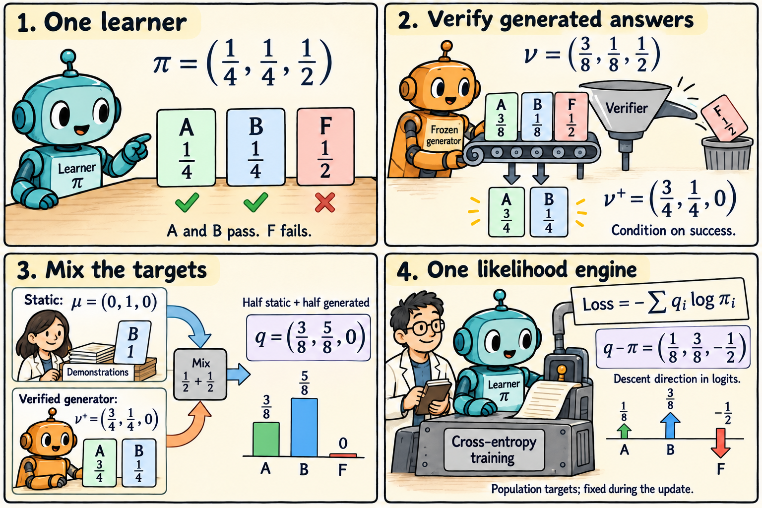
Coordinates are ordered A, B, F. Both A and B are valid answers; F fails. The comic uses population targets and a frozen generator. Its final vector is a direction in logits, not a vector to add directly to probabilities.
Derive the shared update
Consider one prompt with three possible one-token completions. Let their logits be (z=(z_A,z_B,z_F)), and define the learner’s probabilities by softmax:
\[\pi_i(z)=\frac{e^{z_i}}{\sum_j e^{z_j}},\qquad \ell(z;q)=-\sum_i q_i\log\pi_i(z).\]Here (q) is any fixed probability target. Since (\partial\log\pi_i/\partial z_j=\mathbf{1}{i=j}-\pi_j), summing against (q_i) gives
\[\frac{\partial\ell}{\partial z_j} =-q_j+\pi_j\sum_iq_i=\pi_j-q_j.\]Thus gradient descent takes a logit step (z\leftarrow z+\eta(q-\pi)). A corpus example, a demonstration, and a distribution over verified generations can all enter through (q). The trainer still needs to know which positions are predicted and how their losses are weighted.
For several sources with fixed nonnegative weights summing to one, linearity yields
\[q=\sum_s\lambda_s q_s, \qquad \ell(z;q)=\sum_s\lambda_s\ell(z;q_s), \qquad -\nabla_z\ell=q-\pi.\]For multiple prompts, apply this identity to the joint prompt–completion distribution. Nothing in the identity chooses the source weights, creates useful answers, or verifies them. Those decisions determine the target.
Build the target explicitly
Let the current learner, an independently specified frozen generator, and a static demonstration source be
\[\pi=\left(\frac14,\frac14,\frac12\right),\qquad \nu=\left(\frac38,\frac18,\frac12\right),\qquad \mu=(0,1,0).\]Take fixed rewards (r(A)=r(B)=1) and (r(F)=0). The generator succeeds with probability (p_\nu=3/8+1/8=1/2). Conditioning its output on success gives
\[\nu^+=\left(\frac{3/8}{1/2},\frac{1/8}{1/2},0\right) =\left(\frac34,\frac14,0\right).\]An equal mixture of the static and generated population targets is therefore
\[q=\frac12\mu+\frac12\nu^+ =\left(\frac38,\frac58,0\right), \qquad d=q-\pi=\left(\frac18,\frac38,-\frac12\right).\]The static source teaches B, while the verified generator favors A over B by three to one. Their mixture favors B, five to three. This is a concrete statement about the learning signal that a source proportion produces. It cannot be inferred from the label “post-training” alone.
The direction sums to zero, as softmax’s invariance to a common logit shift requires. It also decreases the failed answer’s logit relative to both successful answers in this particular example. Finite steps still pass through softmax; the fractions in (d) are not probability increments.
Locate the RL equivalence
For on-policy binary rewards with positive success probability, fitting the current policy’s success-conditioned target yields MaxRL’s gradient at the current parameters. A different generator supplies its own target. REINFORCE also requires prompt reweighting and the corresponding scale. Section 3; Appendix F.1.
For our learner, the on-policy successful target would be (\pi^+=(1/2,1/2,0)). The pure generated-data descent directions differ:
| Target source | Direction in logits |
|---|---|
| Current learner’s successful answers | ((1/4,1/4,-1/2)) |
| Frozen generator’s successful answers | ((1/2,0,-1/2)) |
Both generators have success probability one half, but they divide their successful mass differently. An old or external generator can therefore change the update even when its pass rate matches the learner’s. A zero B component in the second row only means its logit has zero instantaneous change; its probability can change through the denominator.
The gradient identity can also be checked directly. With a parameter-independent success set and (p_z=\pi_A+\pi_B>0),
\[\nabla_z\log p_z =\frac{1}{p_z}\sum_{i\in\{A,B\}}\nabla_z\pi_i =\sum_{i\in\{A,B\}}\frac{\pi_i}{p_z}\nabla_z\log\pi_i.\]This evaluates scores at the current learner and weights them with its own conditional distribution. Replacing those weights by another generator’s conditional distribution changes the expression. Likewise, rebuilding the target after a parameter change differs from repeatedly fitting the old target. A fixed-target derivative should not silently differentiate through the process that created the target.
Two samples change the effective mixture
The implementation uses weighted token losses, reward verification and asynchronous generation. Its finite-sample rule assigns no update to all-failure groups. Section 4.
We can quantify the consequence without a language model. Keep the one-token responses above, draw two independent completions from (\nu), and average the scores of successful answers within a group. Use zero when both fail. The three possible success counts have probabilities
\[\Pr(M=0)=\frac14,\qquad \Pr(M=1)=\frac12,\qquad \Pr(M=2)=\frac14.\]Conditional on either positive count, the successful-answer average has expectation (\nu^+-\pi). Hence the expected generated-data direction is only (\Pr(M>0)(\nu^+-\pi)=\tfrac34(\nu^+-\pi)).
Suppose half the update groups are static and half are these two-sample generated groups, with the same outer weighting. Retain all-failure groups in that accounting. Then
\[\begin{aligned} \bar d &=\frac12(\mu-\pi)+\frac12\frac34(\nu^+-\pi)\\ &=\left(\frac1{16},\frac38,-\frac7{16}\right)\\ &=\frac78\left[ \left(\frac9{28},\frac{19}{28},0\right)-\pi \right]. \end{aligned}\]There are two effects: an overall gradient scale of (7/8), and an effective generated-target share of ((3/8)/(7/8)=3/7), below the configured one half. Dropping empty groups and renormalizing would define a different sampler. Variable response lengths and token normalization introduce further changes; this calculation assumes equal lengths and the stated group averaging.
More generally, with (N) independent attempts and success probability (p>0), a group contributes with probability (1-(1-p)^N). Thus a sampling budget is also a curriculum decision: the generator and verifier jointly determine which prompts yield a training signal. Increasing the nominal RL fraction does not by itself guarantee more effective weight on rarely solved prompts.
Reproduce the fractions
This enumeration includes all nine ordered pairs of generated outcomes, including failure–failure:
from fractions import Fraction as F
from itertools import product

pi = (F(1, 4), F(1, 4), F(1, 2))
nu = (F(3, 8), F(1, 8), F(1, 2))
mu = (F(0), F(1), F(0))
target = (F(3, 4), F(1, 4), F(0))
q = tuple((a + b) / 2 for a, b in zip(mu, target))
d = tuple(a - b for a, b in zip(q, pi))
generated = [F(0)] * 3
for i, j in product(range(3), repeat=2):
    passed = [k for k in (i, j) if k != 2]
    if not passed:
        continue  # zero contribution, not resampled
    for k in range(3):
        score = F(passed.count(k), len(passed)) - pi[k]
        generated[k] += nu[i] * nu[j] * score
finite = tuple((mu[k] - pi[k] + generated[k]) / 2
               for k in range(3))
assert d == (F(1, 8), F(3, 8), F(-1, 2))
assert finite == (F(1, 16), F(3, 8), F(-7, 16))
What to optimize next
The paper studies 124M and 0.76B models. Accuracy, coverage and retention trade off across mixtures. Its compute frontiers compare evaluated configurations; they are not universal scaling laws. Sections 5 and 7; Appendix A.2. The likelihood identities do not automatically cover PPO’s or GRPO’s clipping and penalties. Appendix F.1.
My research judgment is that the most useful next experiment would control effective target exposure, rather than just the configured static/RL percentage. Log generator versions, per-prompt success-group rates, response lengths, realized source contributions and fresh-generation cost. Compare schedules at matched compute and report accuracy, coverage and retention separately.
For federated or asynchronous learning, a further question is who supplies the successful answers. Two clients can have equal pass rates but incompatible distributions over valid solutions, just like the two generators above. Balancing their example counts does not balance the directions they teach. A useful controller would need to track that distributional disagreement as well as age and yield.
The shared loss is an organizing principle for these questions. It does not establish convergence for adaptive mixtures, guarantee that an arbitrary generator improves the current policy’s reward, or make a verifier’s mistakes harmless. Keeping the learner’s objective simple makes the design of the target distribution more consequential.
Sources
Yuda Song, Alvin Zhang, Fahim Tajwar, Daman Arora, Jeff Schneider, Daniel Khashabi, Ruslan Salakhutdinov, J. Andrew Bagnell, Aarti Singh and Andrea Zanette. Training Foundation Models with a Single Algorithm. arXiv:2610.40564v1, first public 29 October 2026. Full text, especially Sections 3–4 and Appendices A and F. The three-outcome mixture, finite-sample calculation and proposed research controls above are original worked analysis.
The comic was created with AI.