A server merging two neural networks has to decide which hidden neurons belong together before averaging their parameters. A consistent swap of hidden neurons and their outgoing connections preserves the network’s predictions, so upload order alone gives a weak basis for this decision. In one-shot federated learning, the server has one opportunity to make the merge. FedFiOT uses the same Fisher-weighted cost to choose neuron correspondences and to compute their merged weights. In the example below, both steps are exact, yet the starting reference determines which of two fixed points the server reaches. Nguyen et al., FedFiOT, arXiv:2611.06783v1.
What the server minimizes
Fix a layer and a common ordering of its incoming coordinates. Let \(x_{kj}\) be client \(k\)’s weight vector for neuron \(j\), \(w_i\) the server’s vector in slot \(i\), and \(\pi_k(i)\) the client neuron assigned to that slot. The clients share the same layer width. The diagonal precision matrix \(D_{kj}\) moves with the client neuron. Each diagonal entry is a mean squared per-example log-likelihood derivative using observed labels, raised to a power \(0<\rho\leq 1\) and then increased by \(\lambda>0\). The empirical diagonal supplies a local sensitivity proxy. Section 3.2 and Equation (2), Appendix B and Equation (102).
\[J(w,\pi)=\sum_{k,i}(w_i-x_{k,\pi_k(i)})^\top D_{k,\pi_k(i)}(w_i-x_{k,\pi_k(i)}).\]At fixed \(w\), each client solves a linear assignment. Dividing a permutation matrix by the layer width gives a transport plan with uniform marginals. Every plan with those marginals is a convex combination of such plans, so an exact assignment reaches the optimal linear transport cost. At fixed permutations, differentiating in each slot gives a linear system whose coefficient matrix is the sum of the matched precisions. Its solution is a coordinatewise precision-weighted average. Damping gives that quadratic block Hessian a lower bound of \(2K\lambda I\) for \(K\) clients. Thus an iteration lowers the fixed-layer objective by at least \(K\lambda\lVert w^{[s]}-w^{[s-1]}\rVert^2\). Summing this inequality bounds the smallest step in the first \(S\) iterations at order \(S^{-1/2}\). Section 3.3, Equations (4)–(7), Theorem 1 and its proof.
Two starting references
Take one layer, two clients and two scalar neurons per client. With \(\lambda=1\), client A uploads weights \((1,6)\) with damped precisions \((1,1)\). Client B uploads \((0,1)\) with damped precisions \((1,4)\). These are toy inputs to the layer objective. For a pair of scalar weights \(x,y\) with precisions \(p,q>0\), completing the square gives
\[p(w-x)^2+q(w-y)^2 =(p+q)\left(w-\frac{px+qy}{p+q}\right)^2 +\frac{pq}{p+q}(x-y)^2.\]The last term is the cost of a pairing after the server optimizes the merged weight. It lets us compare the two relative permutations directly.
- Start from B’s weights \((0,1)\). B keeps its own order at zero cost. A’s direct assignment costs \(1+25=26\) and its swap costs \(36\). The merge is \((1/2,2)\) and the minimized cost is \(1/2+20=41/2\). At that merge, switching A alone adds \(15\) and switching B alone adds \(3/4\), so the next assignment keeps both in place.
- Start from A’s weights \((1,6)\). A keeps its order at zero cost. For B, keeping its order costs \(1+4\cdot25=101\), while swapping costs \(36\). With B’s precisions swapped along with its weights, the merge is \((1,3)\). The first pair has zero discrepancy and the second costs \(36/2=18\). Switching A alone at that merge adds \(20\) and switching B alone adds \(8\).
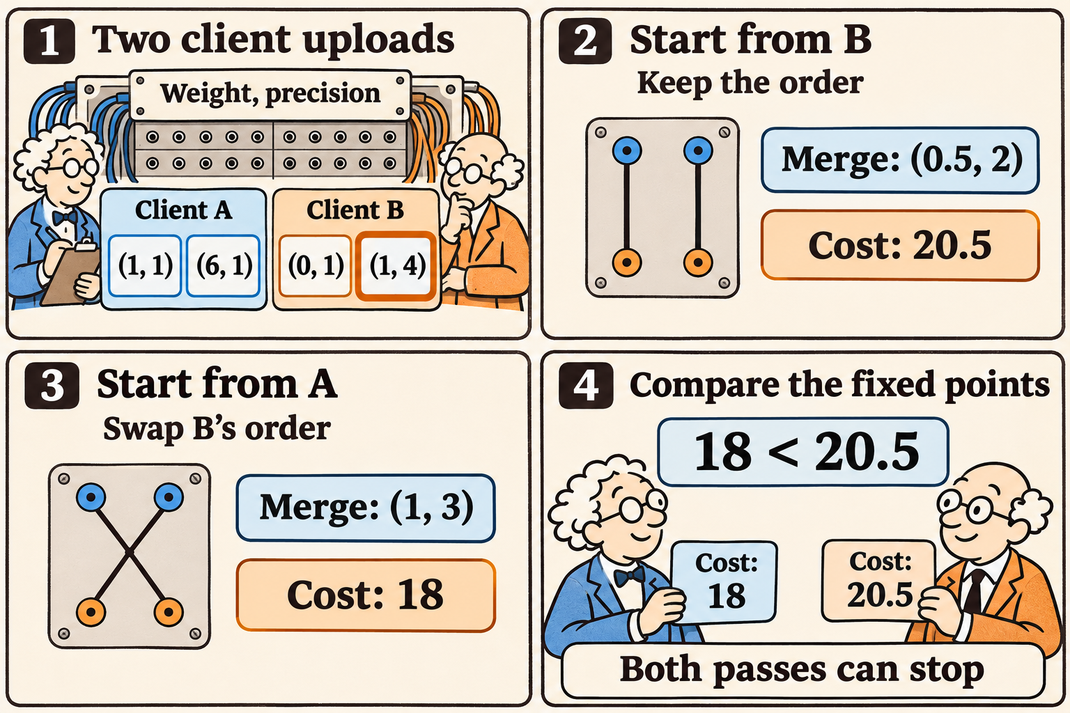
The straight and crossed wires show the two possible relative pairings. Reversing the global slot order and both clients’ assignments together just relabels the same solution, so \(18\) is the global minimum of this layer toy. The identity-aligned fallback has cost \(20.5\). It keeps the lower-cost candidate when the solver starts from A, and yields the identity result when the solver starts from B. Exact descent can stop with a gap of \(5/2\).
The same example separates the effect of damping on the first assignment from its effect on the best reoptimized pairing. Hold the undamped precisions at \((0,0)\) and \((0,3)\), respectively, and vary \(\lambda\). Starting from A, B’s two assignment costs are \(26\lambda+75\) for the direct wires and \(36\lambda\) for the crossed wires. That preference switches at \(15/2\). After optimizing the merged weights under both pairings, the cost gap is
\[J_{\rm direct}^{\star}-J_{\rm cross}^{\star} =\frac{5\lambda(9-4\lambda)}{2(2\lambda+3)}.\]The reoptimized preference switches earlier, at \(9/4\). For instance, at \(\lambda=3\), starting from A favors crossing (\(108\) versus \(153\)), while the optimized direct and crossed costs are \(51.5\) and \(54\). A damping sweep therefore changes the discrete optimization problem as well as the weighted means.
What would justify a second start?
The training guarantee addresses a different question. It bounds the average expected squared gradient norm of the equal-client loss under full participation, smooth lower-bounded optimization, fresh bounded and unbiased stochastic gradients, bounded client heterogeneity and Fisher entries, loss-preserving permutations, and a small effective local step. The identity comparison controls aligned dispersion using \(\kappa=(F_{\max}+\lambda)/\lambda\). Unequal normalized Fisher weights can leave a residual in the stationarity bound through that dispersion. The comparison itself is in the quadratic merge objective. Its usefulness for predicting test accuracy remains empirical. Section 4.2, Equations (17)–(22).
The authors evaluate a small CNN on three image datasets, with synthetic label skew, three training seeds on a fixed partition, and a 500-example server validation set. On CIFAR-10 at a Dirichlet concentration of \(0.1\), Table 1 reports one-shot mean accuracy of 43.3% for FedFiOT and 38.6% for FedFisher with K-FAC. Quantizing weights and diagonal Fishers to 16 bits each gives an upload of \(32d+64L\) bits for \(d\) parameters and \(L\) layers, including the layer scales. Computing the empirical Fisher still adds a pass over local data, and the exact matching cost grows cubically with layer width once the cost matrix is built. Section 5, Appendix C.
A useful test would reuse each round’s uploads and compare the paper’s largest-client reference with two additional trained-client references, keeping damping and the local training budget fixed. Select the candidate with the lowest full-model merge cost, including the identity candidate, and report the spread in merge cost, class-balanced held-out loss and server time across independent partitions. This would show whether extra starts pay for themselves under severe label skew and whether a better surrogate score predicts better performance on rare classes.
The comic was created with AI.