A Faster Rate to a Shifted Target

Adding curvature can make a convergence theorem much stronger while moving the point that the algorithm approaches. Cortild and Cartis study this tradeoff through a random positive quadratic added to an arbitrary objective. For gradient descent, their smoothed analysis recovers a logarithmic dependence on relative accuracy over a class of convex problems that may have zero curvature. The accuracy is measured on the perturbed objective. This matters when applying the result to an empirical training loss whose minimizer is the quantity of interest. Cortild and Cartis, From Worst-Case to Smoothed Complexity in Continuous Optimization, arXiv:2611.14282v1, Sections 3–3.1.

Write \(r=\sigma^2>0\). Draw \(W=GG^\top/m\) once, where \(G\) has \(n\) rows, \(m\) columns and independent standard Gaussian entries. Fix the scale, starting point and center \(c\) before that draw and optimize

For convex \(f\) with an \(L\)-Lipschitz gradient, valid curvature bounds are \(\mu_r=r\lambda_{\min}(W)\) and \(L_r=L+r\lambda_{\max}(W)\). Gradient descent uses step \(1/L_r\). In the proportional growth regime \(n/m\to d\in(0,1)\) from below, with \(n/m\leq d\), Theorem 3.2 bounds expected iterations to relative gap \(\varepsilon\) by \(1+O_d((1+L/r)\log(1/\varepsilon))\). The matrix stays fixed during each run. Equations (1)–(2) and Theorem 3.2.

Here is the mechanism behind that bound. Smoothness and the step choice give \(h(x^+)\leq h(x)-\lVert\nabla h(x)\rVert^2/(2L_r)\). Strong convexity gives \(\lVert\nabla h(x)\rVert^2\geq2\mu_r(h(x)-\min h)\). Combining them yields a gap contraction by \(1-\mu_r/L_r\), so the iteration bound involves the ratio \(L_r/\mu_r\). Taking an expectation requires control of inverse eigenvalues and of the ratio of extreme eigenvalues. Knowing the average added curvature alone leaves this ratio undetermined. The paper supplies the necessary moment bounds under its aspect ratio and dimension assumptions. Theorem 2.1, Proof 3.3.

Consider a concrete perturbation in two dimensions. Let \(f(x)=\tfrac12(x_1-1)^2\), \(c=(0,0)\), \(r=1/3\) and \(W=\begin{pmatrix}2&1\\1&2\end{pmatrix}\). This is a deterministic illustration of the quadratic perturbation mechanism. The original Hessian has eigenvalues zero and one. The added matrix has eigenvalues one and three, giving the valid bounds \(\mu_r=1/3\) and \(L_r=2\). The perturbed Hessian and first-order optimality system are

The actual Hessian eigenvalues are \((7-\sqrt{13})/6\) and \((7+\sqrt{13})/6\), both positive. Thus the generic bound gives a geometric gap factor \(5/6\) for step \(1/2\). The actual quadratic may converge faster than that conservative bound.

Start at \(x_0=(1,0)\), which already minimizes the original objective. The perturbed gradient there is \((2/3,1/3)\). One step of size \(1/2\) gives \(x_1=(2/3,-1/6)\). Solving the displayed system gives the new minimizer \(x_r=(2/3,-1/3)\). At the start, \(h(x_0)=1/3\). After one step, \(h(x_1)=19/108\), and at the new minimizer, \(h(x_r)=1/6\). The perturbed gap has fallen from \(1/6\) to \(1/108\) in one step. Meanwhile, the original loss has risen from zero to \(1/18\) and remains \(1/18\) at \(x_r\).

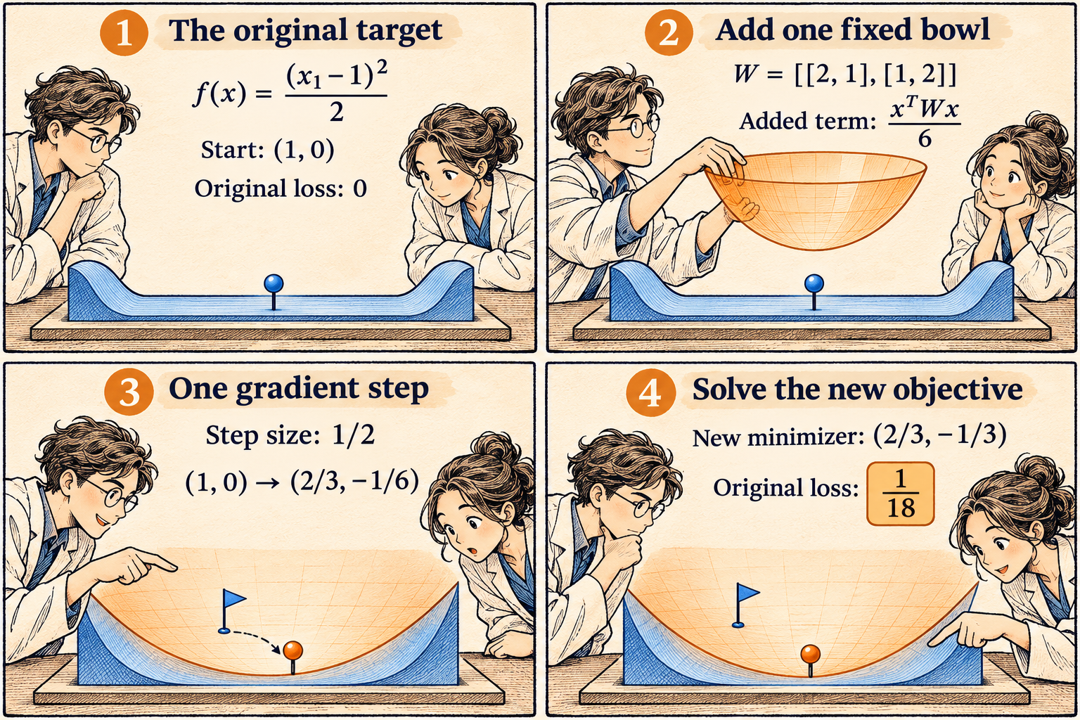
The flat valley in the comic represents the original set of minimizers. The added bowl creates a unique destination. The separated markers in the final panel show the displacement. This example isolates the accuracy effect by starting from an original minimizer.

The source gives a direct way to account for the displacement. If \(x_*\) minimizes \(f\) and \(h(x)-\min h\leq\delta\), then nonnegativity of the quadratic and \(\min h\leq h(x_*)\) imply

For the toy, the rightmost term is \(1/3\) when \(x_*=(1,0)\), compared with the actual limiting original loss \(1/18\). The bound is conservative, but it exposes the dependence on the perturbation center. For a fixed original minimizer and center, \(\mathbb E W=I\) also gives an expected bias allowance of \(r\lVert x_*-c\rVert^2/2\). Perturbation bias bound in Section 3.

An absolute accuracy requirement changes how the convergence bound should be read. For one fixed matrix, suppose \(\lVert x_*-c\rVert\leq R\) and \(\lambda_{\max}(W)\leq M\). Choosing \(\delta=\epsilon/2\) and \(r=\epsilon/(MR^2)\), for \(R>0\), makes the displayed original-loss bound at most \(\epsilon\). With this sufficient choice, the condition-number bound becomes \(LMR^2/(\epsilon\lambda_{\min}(W))+\lambda_{\max}(W)/\lambda_{\min}(W)\). Shrinking the permitted bias therefore places an inverse-accuracy factor outside the logarithm. This conversion is a sufficient guarantee, whose tightness depends on the objective and center.

For learning applications, I would compare perturbation scales at the same original-loss threshold, tracking both objectives and the distance from the perturbation center. Repeat the matrix draws at several aspect ratios and include matrix construction and multiplication in runtime. The paper’s numerical illustrations average over 100 draws and show that the theoretical bounds can be pessimistic for actual iteration counts. Measuring original-loss accuracy as well would establish where the added curvature pays for its displacement and computation. Numerical setup and GD illustrations.

The comic was created with AI.