A sign optimizer discards the gradient’s magnitude, yet its average update can still respond to curvature. Noise supplies the scale: a small gradient wins the sign vote more often when the noise around it is small. Wang and colleagues develop this mechanism into a functional scaling law for a continuous model of SignSGD in kernel regression. Their analysis connects faster learning of weak spectral directions with a persistent cost from noisy updates. When and How SignSGD Outperforms SGD: A Functional Scaling Law Perspective, arXiv:2611.16560v1.
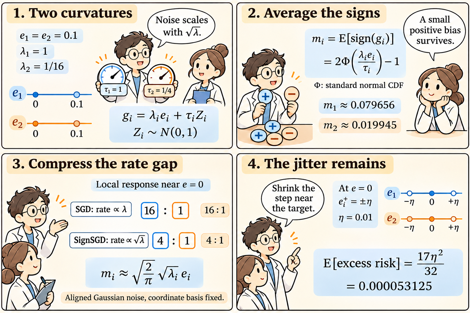
Start with a finite quadratic example that can be calculated directly. Write the parameter error as \(e=\theta-\theta^*\) and excess risk as \(\mathcal E(e)=\tfrac12\sum_i\lambda_i e_i^2\), with positive curvatures \(\lambda_i\). Suppose a stochastic gradient coordinate is \(g_i=\lambda_i e_i+\tau_i Z_i\), where the \(Z_i\) are independent standard normal variables and \(\tau_i>0\) is the noise standard deviation. A SignSGD step is \(e_i^+=e_i-\eta\operatorname{sign}(g_i)\) with step size \(\eta>0\). If \(\Phi\) denotes the standard normal cumulative distribution function, the probability of a positive gradient is \(\Phi(\lambda_i e_i/\tau_i)\). Therefore its mean sign and variance are exactly
\[\begin{aligned} m_i(e_i)&:=\mathbb E[\operatorname{sign}(g_i)] =2\Phi(\lambda_i e_i/\tau_i)-1,\\ \operatorname{Var}(\operatorname{sign}(g_i))&=1-m_i(e_i)^2. \end{aligned}\]The expected displacement is \(-\eta m_i(e_i)\). Around zero error, differentiating the Gaussian CDF gives \(m_i(e_i)=\sqrt{2/\pi}(\lambda_i/\tau_i)e_i+O(e_i^3)\) for fixed curvature and noise. If \(\tau_i=\sqrt{\lambda_i}\), the linear coefficient is proportional to \(\sqrt{\lambda_i}\). Plain SGD’s mean response has coefficient \(\lambda_i\). This calculation concerns the local mean response; individual sign updates retain magnitude \(\eta\). It is the scalar mechanism used in the paper’s Section 6.1.
Take \(\lambda=(1,1/16)\), \(\tau=(1,1/4)\) and \(e=(0.1,0.1)\). The mean gradients are \((0.1,0.00625)\), a ratio of sixteen. The gradient-to-noise ratios are \((0.1,0.025)\), giving \(m_1\approx0.079655675\) and \(m_2\approx0.019945036\). Their ratio is approximately \(3.993759\). As the equal errors approach zero, the mean sign ratio tends to four. The slow coordinate receives a larger relative mean response. A learning rate comparison and the update variance are still needed to turn that observation into a risk comparison.
The same calculation exposes the cost. Squaring the actual update, using \(\operatorname{sign}(g_i)^2=1\) almost surely, and then taking expectation yields the exact one-step identity
\[\mathbb E[\mathcal E(e^+)\mid e] =\mathcal E(e)-\eta\sum_i\lambda_i e_i m_i(e_i) +\frac{\eta^2}{2}\sum_i\lambda_i.\]At the optimum, the improvement term vanishes. Each coordinate moves by \(+\eta\) or \(-\eta\) with equal probability. In our example the expected excess risk after one step is \(17\eta^2/32\). With \(\eta=0.01\), this is exactly \(17/320000=0.000053125\), starting from zero risk. For comparison, SGD with the same gradient oracle has one-step risk
\[\mathbb E[\mathcal E(e^+_{\mathrm{SGD}})\mid e] =\frac12\sum_i\lambda_i\left[(1-\eta\lambda_i)^2e_i^2+\eta^2\tau_i^2\right].\]At the optimum its noise contribution is \(257\eta^2/512\), versus SignSGD’s \(272\eta^2/512\). These fixed-step numbers isolate the noise cost in this toy; each optimizer can choose its own schedule.
The coordinate basis is another essential condition. Rotate both the Hessian and noise covariance of this example by forty-five degrees. They remain equal. Both coordinate noise variances become \(17/32\), so the local mean sign map has Jacobian \(J_{\mathrm{sign}}\) given by
\[\begin{aligned} H'=\Sigma'&=\frac1{32}\begin{pmatrix}17&15\\15&17\end{pmatrix},\\ J_{\mathrm{sign}}&=\sqrt{2/\pi}\,\operatorname{diag}(\Sigma')^{-1/2}H'\\ &=\sqrt{2/\pi}\sqrt{32/17}\,H'. \end{aligned}\]Its eigenvalue ratio remains sixteen. The unrotated ratio was four. Curvature alignment alone therefore does not ensure a square-root spectrum when sign acts in a fixed coordinate basis. This rotation calculation explains why the paper separately requires diagonal features. Correlated noise after rotation also prevents treating the sign-update noise as independent across coordinates.
To connect the toy to scaling, suppose the eigenvalues follow \(\lambda_j\asymp j^{-q}\) with \(q>1\), and initial signal energies follow \(\lambda_j\lvert\theta_j^*\rvert^2\asymp j^{-1-sq}\) with \(s>0\). Here \(\asymp\) means bounded above and below by fixed positive multiples. A local decay rate proportional to \(\sqrt{\lambda_j}\) places the spectral frontier at \(j_t\asymp t^{2/q}\). The remaining signal tail is of order \(j_t^{-sq}=t^{-2s}\). Near zero, independent Gaussian sign noise has variance approaching one in every coordinate, so its risk-weighted tail is of order \(\sum_{j>j_t}\lambda_j\asymp j_t^{1-q}=t^{-(2-2/q)}\). In the corresponding SGD model, rates proportional to \(\lambda_j\) give frontier \(t^{1/q}\), while curvature-aligned update noise contributes weights proportional to \(\lambda_j^2\). Its signal and noise tails have orders \(t^{-s}\) and \(t^{-(2-1/q)}\). The slower aggregate noise-forgetting law for SignSGD reflects the changed noise weights as well as the changed decay rates.
The paper makes the SignSGD comparison rigorous for its nonlinear stochastic differential equation (SDE). Its risk is comparable to \(S(t)+\int_0^tK(t-u)n_B(u)\,du\), with \(S(t)\asymp(1+t)^{-2s}\) and \(K(t)\asymp(1+t)^{-(2-2/q)}\). For batch size \(B\) and continuous step variable \(z\), intrinsic time is \(t=\Gamma_B(z)=\sqrt B\int_0^z\eta(v)\,dv\) and noise intensity is \(n_B(t)=\eta(\Gamma_B^{-1}(t))/\sqrt B\). The theorem assumes zero initialization, constant-order label noise, the infinite power-law spectrum, diagonal curvature and fixed Gaussian noise covariance comparable to the Hessian. It also requires \(\sqrt B\sup_z\eta(z)\lesssim1\) and \(t\gtrsim B^{\max\{1/2,1/(2s+2/q)\}}\). Theorem 3.1.
The proof does more than linearize at zero. It rescales each coordinate, bounds its second moment from below using a quadratic test function, and obtains an upper bound with a function that is quadratic locally and exponential in the tails. The burn-in condition absorbs large initial errors before summing over spectral modes. The resulting bounds belong to the SDE; matching discrete conditional means and covariances does not establish a finite-step approximation error. The original regression gradient also has state-dependent, generally non-Gaussian noise. Appendix D, Appendix C.5.
My research takeaway is to test noise geometry before interpreting normalization as acceleration. Estimate coordinate noise scales, compare their relation to curvature, and repeat the comparison under rotations while retuning each optimizer’s schedule. Those controls separate the proposed mechanism from a convenient coordinate system. The paper’s language-model loss-curve fits offer evidence for prediction across schedules and batch sizes; its Adam extension is heuristic. Neither supplies a general optimization guarantee for evolving neural-network geometry. The useful hypothesis is precise enough to challenge: weak directions should gain relative mean drift when coordinate noise tracks curvature, and that gain must pay for the noise introduced near the target. Experiments and scope, Adam discussion.
The comic was created with AI.