Model consensus and gradient similarity measure different things. Two nearby models may be evaluated on different data. A two-node calculation using Decentralized Primal Averaging (DPA) makes the distinction concrete. Ghaderyan and Werner, DPA, arXiv:2611.16871v1.
For deterministic scalar nodes, \(y,x,z,u\) denote optimization, output, evaluation and momentum, stacked into columns. The objective is \(f=n^{-1}\sum_i f_i\). With symmetric doubly stochastic \(W\), fixed \(a,b,\beta_1,\beta_2\in(0,1)\) and \(\eta>0\), DPA uses
\[\begin{aligned} z^k&=b y^k+(1-b)x^k,\\ g_i^k&=f_i'(z_i^k),\\ y^{k+1}&=W\bigl[y^k-\eta(\beta_1u^k+g^k)\bigr],\\ u^{k+1}&=(1-\beta_2)u^k+\frac{\beta_2}{\eta}(y^k-y^{k+1}),\\ s^k&=(1-a)x^k+a y^{k+1},\\ x^{k+1}&=Ws^k. \end{aligned}\]The two \(W\) multiplications communicate model-sized vectors; momentum stays local. Algorithm 1, Equations (2)–(5).
Consider two deterministic objectives \(f_1(t)=(t-1)^2/2\) and \(f_2(t)=(t-3)^2/2\). Their average is \(f(t)=(t-2)^2/2+1/2\), minimized at two. Use
\[W=\begin{pmatrix}3/4&1/4\\1/4&3/4\end{pmatrix}, \qquad x^0=y^0=u^0=(0,0)^\top.\]Set \(\eta=1\) and \(a=b=\beta_1=\beta_2=1/2\). These parameters give a finite-step illustration of Algorithm 1 chosen for hand calculation. They lie outside the convergence theorem’s sufficient learning-rate and momentum conditions. The objectives themselves have smoothness \(L=1\), zero stochastic variance and uniformly bounded heterogeneity \(\zeta^2=1\), since their gradients differ from the global gradient by \(+1\) and \(-1\) everywhere.
At the first evaluation, \(z^0=(0,0)^\top\) and \(g^0=(-1,-3)^\top\). The local proposal is \(v^0=(1,3)^\top\), because the momentum buffer starts at zero. The first gossip gives \(y^1=Wv^0=(3/2,5/2)^\top\). The buffer becomes \(u^1=(-3/4,-5/4)^\top\), and local output averaging gives \(s^0=y^1/2=(3/4,5/4)^\top\). The second gossip produces \(x^1=Ws^0=(7/8,9/8)^\top\). Its mean is one, the same as the mean of \(s^0\); the node-to-node gap shrinks from \(1/2\) to \(1/4\).
To isolate this second mixing step, form a control that instead keeps \(x^1=s^0\), holding all preceding calculations fixed. At the next evaluation, both branches use \(z^1=(y^1+x^1)/2\). Full DPA gives \(z^1=(19/16,29/16)^\top\), while the control gives \(z^1=(9/8,15/8)^\top\). The evaluation-point gap is smaller with the extra gossip: \(5/8<3/4\). Yet the corresponding local gradients are \((3/16,-19/16)^\top\) and \((1/8,-9/8)^\top\). Their absolute gaps satisfy \(11/8>5/4\). Both gradient means equal \(-1/2\). Our control removes only the second gossip.
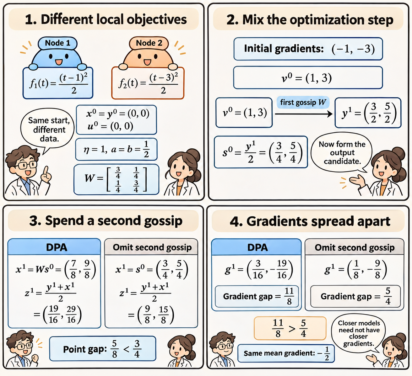
The reason is visible without running another update. Write two evaluation points as \(z_1=m-d\) and \(z_2=m+d\), with \(d\geq0\). Their mean gradient is \(m-2=f'(m)\), while the deviations from that mean are \(1-d\) and \(-(1-d)\). Thus the mean squared model disagreement is \(d^2\) and the mean squared local gradient dispersion is \((1-d)^2\). For \(0<d<1\), reducing the first quantity increases the second. In our two branches, \(d\) falls from \(3/8\) to \(5/16\): model disagreement falls from \(9/64\) to \(25/256\), while gradient dispersion rises from \(25/64\) to \(121/256\). At exact consensus, \(d=0\), model disagreement is zero but gradient dispersion remains one. If both nodes instead had the same quadratic centered at two, gradient dispersion would equal \(d^2\). The different local objectives create the reversal.
This example establishes no improvement in the average optimization direction: both branches have \(m=3/2\) and the same global gradient there. It also says nothing about their eventual convergence or test accuracy. Its value is diagnostic. A raw measure of local gradient similarity can move in the opposite direction from model consensus, even when communication contracts the model gap exactly.
A shifted iterate and weighted consensus Lyapunov bound control stationarity. Assumptions include a fixed synchronous network with positive mixing gap, smoothness, conditionally independent unbiased bounded-variance gradients, uniform bounded heterogeneity, a lower-bounded objective, consensus initialization, bounded coefficients and parameter restrictions. Appendix B, Appendix C.
For constant-within-run \(\eta=c\sqrt{n/T}\) satisfying those restrictions, DPA bounds time-averaged expected squared global gradients at the average output by \(\tfrac73[D_1/\sqrt{nT}+D_2n/T]\). This covers neither the last iterate nor DPA-1G. Corollary 2, Remark 3.
With \(D_1>0\), requiring the residual term to be no larger than the leading term gives \(T\geq(D_2/D_1)^2n^3\) by squaring \(D_2n\sqrt n\leq D_1\sqrt T\). The bound’s network-dependent constants and admissible parameters must also be tracked as the graph grows. A statement about the global gradient does not require each local objective’s gradient to vanish: at our global optimum two, those local gradients are \(+1\) and \(-1\).
My research judgment is to compare these methods at a communication budget while recording three distinct measurements: model disagreement, local gradient dispersion and global stationarity. The toy explains why one cannot substitute for another. DPA’s second output mix affects the next training query, so its role extends beyond smoothing a model at evaluation time. A useful next experiment would hold the number of gradient queries and gossip rounds fixed, but move the second gossip from the output sequence to the optimization sequence in a control. Repeating that comparison as local objectives become more different would test the value of where the communication is spent within the coupled dynamics. The paper’s communication comparisons provide a starting point.
The comic was created with AI.