When two prediction distributions nearly agree, their KL divergence is a second-order quantity assembled from first-order terms. An ordinary-looking sum can therefore erase the signal it is supposed to measure. The binary example below returns zero even in double precision, although every input probability is stored exactly.
Brandon Amos’s On numerical issues of divergences between nearly equal distributions, first public on November 13, studies categorical divergences and their derivatives. Its useful distinction is between numerical cancellation and the statistical behavior of sampled penalties. Section 4.1 uses an exponential remainder; Section 4.3 separately analyzes sampled values and gradients.
Let \(p_i,q_i>0\) be normalized categorical probabilities, with \(p\) fixed. Define
\[s_i=\log(q_i/p_i),\qquad D=\operatorname{KL}(p\parallel q)=-\sum_i p_i s_i.\]Re-derive the remainder identity by setting \(E_2(x)=e^x-1-x\). Normalization gives
\[\sum_i p_i E_2(s_i) =\sum_i q_i-\sum_i p_i-\sum_i p_i s_i =D.\]Each remainder is nonnegative. Near zero it starts at quadratic order:
\[E_2(x)=x^2\left(\frac12+\frac{x}{6}+\frac{x^2}{24}+\cdots\right), \qquad E_2'(x)=\operatorname{expm1}(x).\]The paper evaluates this remainder through a near-zero series. Writing expm1(x) - x still subtracts nearly equal first-order quantities. Accurate log-ratios and an accurate backward calculation also matter; a positive output alone certifies neither.
To see the geometry without a large vocabulary, consider the following family, with \(0<t<1\):
\[p=(1/2,1/2),\qquad q=((1+t)/2,(1-t)/2).\]The exact divergence reduces to
\[D(t)=-\frac12\log(1-t^2) =\frac{t^2}{2}+\frac{t^4}{4}+\frac{t^6}{6}+\cdots.\]The cancellation is structural: the two signed summands begin at \(-t/2\) and \(+t/2\), while their sum begins at \(t^2/2\). A relative error of size \(u\) in each first-order term can compete with the answer once \(t\) approaches \(u\). Separately rounded logarithms introduce another error scale: their absolute errors can be on the order of \(u\) because the logarithms themselves are near \(-\log 2\). That can obscure a signal of order \(t^2\) much earlier, around \(t\sim\sqrt{u}\). These are conditioning estimates, not universal error bounds for every library.
Take \(t=2^{-27}\). Then \(q=(1/2+2^{-28},1/2-2^{-28})\) has exactly representable binary64 entries and sums exactly to one. For CPython 3.12.14 on Windows x86-64, evaluating \(\tfrac12(\log(1/2)-\log q_i)\) with math.log gives the two rounded terms
The stable binary formula evaluates -0.5 * log1p(-t*t) instead:
This is approximately \(2^{-55}\); the exact divergence is slightly larger. The zero above describes that specified evaluation, rather than every binary64 implementation. Here the information survives input storage and disappears later. Clamping a negative answer to zero would not recover it, and zero itself is already a misleading answer.
For this binary family, the remainder representation is also transparent:
\[D=\frac12 E_2(\log(1+t))+\frac12 E_2(\log(1-t)).\]Using log1p for those log-ratios and a small-argument remainder series preserves the quadratic contributions. The closed binary formula is especially simple; a general categorical implementation needs to retain the log-ratios before evaluating the remainder. Inexact normalization changes the identity by \(\sum_i q_i-\sum_i p_i\), which can itself overwhelm a tiny divergence.
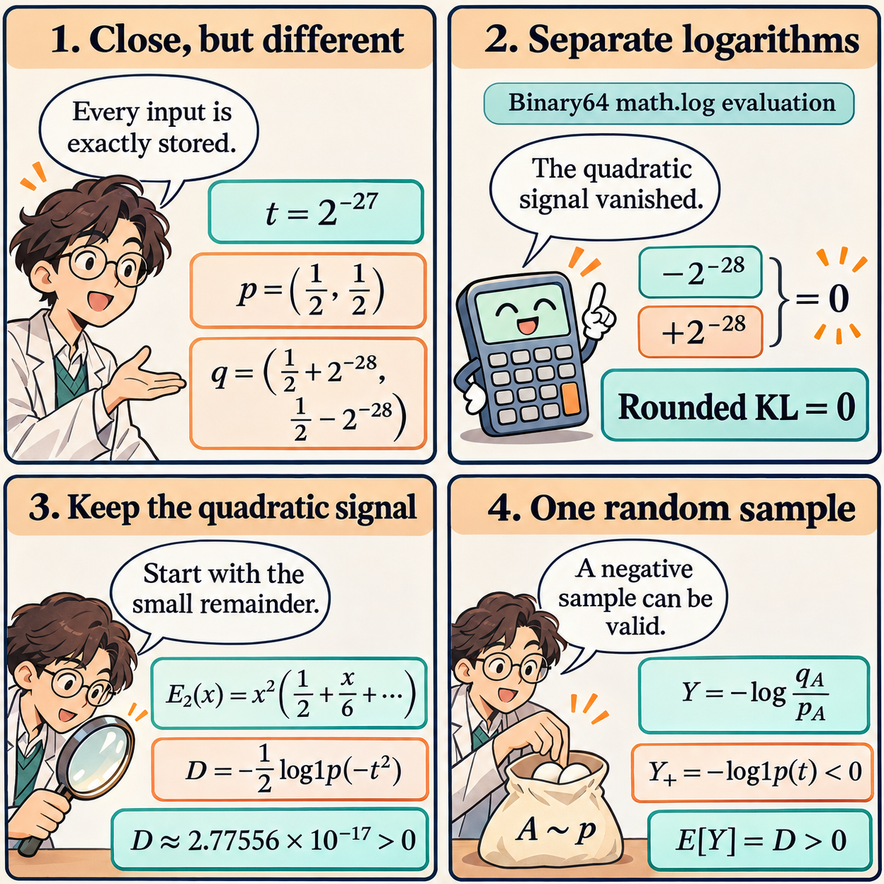
The binary example separates a rounded full sum from a signed random sample. Panel 2 refers to the separate-log binary64 evaluation above; the positive value in panel 3 is approximate.
Now sample one category \(A\sim p\), keeping the same binary family. Let \(s_A=\log(q_A/p_A)\). A single-sample forward-KL estimator is \(Y=-s_A\), so its two possible values are
\[Y_+=-\log(1+t)<0,\qquad Y_-=-\log(1-t)>0.\]Its expectation is exactly \(D(t)\). A negative realization is therefore compatible with a nonnegative divergence even in exact arithmetic. Deriving its variance from the half-difference of the two values gives
\[\operatorname{Var}_p(Y)=\operatorname{atanh}(t)^2, \qquad \operatorname{atanh}(t)=\frac12\log\frac{1+t}{1-t}.\]The nonnegative alternative \(C=E_2(s_A)\) has values \(C_+=t-\log(1+t)\) and \(C_-=-t-\log(1-t)\). Adding the equally likely terms \(+t\) and \(-t\) leaves the expectation unchanged. The same calculation yields
\[\mathbb E_p C=D(t),\qquad \operatorname{Var}_p(C)=(\operatorname{atanh}(t)-t)^2.\]Thus the two variances scale as \(t^2\) and \(t^6/9\) near equality. At \(t=1/5\), both estimators have mean \(\tfrac12\log(25/24)\approx0.0204109973\), but their variances are approximately \(0.0411004885\) and \(0.00000746685166\). This is an exact-family variance reduction, separate from floating-point stability. Computing \(C_\pm\) by those subtractive expressions can still lose accuracy near zero; the remainder series remains relevant.
Values and gradients require another distinction. Parameterize \(q_1=\sigma(\theta)\) and \(q_2=1-q_1\), where \(\sigma\) is the logistic function. For the full forward KL,
\[\frac{d}{d\theta}\operatorname{KL}(p\parallel q)=q_1-\frac12=\frac t2.\]The loss is quadratic in \(t\) while this logit derivative is linear. A small loss value alone therefore says little about whether its derivative was preserved.
For an exact example of an objective mismatch, sample \(A\sim q\) and form the reverse-KL value estimator \(H=E_2(-s_A)=s_A+e^{-s_A}-1\). Its expectation equals \(R=\operatorname{KL}(q\parallel p)\). If the sampled category is held fixed during differentiation, then
\[\mathbb E_q[\partial_\theta H] =\sum_a(q_a-p_a)\partial_\theta\log q_a =q_1-\frac12.\]But differentiating the full reverse KL, including the sampling probabilities, gives
\[\frac{dR}{d\theta}=q_1(1-q_1)\log\frac{q_1}{1-q_1}.\]At \(t=1/5\), these are \(0.1\) and \(0.24\log(1.5)\approx0.0973116259\). The missing sampling-law derivative explains the discrepancy. More precise arithmetic preserves the chosen update; it cannot turn it into a different derivative. The full categorical remainder sum, differentiated through its weights as well, does include that dependence.
My research judgment is that a KL diagnostic near agreement should specify the quantity being computed, its sampling direction, and the derivative actually used. The binary calculation shows why changing the final reduction alone may be insufficient: separately rounded log-probabilities can already have lost the second-order signal. The variance calculation shows a distinct opportunity for improvement before floating-point rounding enters at all. Neither result establishes a downstream training benefit by itself.
The paper’s near-equality formulas are local tools, with explicit range and input-rounding limitations (Section 4.1 and Appendix A). A useful next experiment would isolate log-ratio construction, remainder evaluation, and backward computation while holding the sampling rule fixed. I would expect that separation to be more informative than comparing only nonnegative loss curves. Tiny KL values can be meaningful, provided their numerical and statistical definitions survive the implementation.
The comic was created with AI.