A history vector can be useful because it remembers a combination of old gradients. It can also be useful because it forgets. Those two capabilities lead to different storage counts, even for exactly the same linear update rule.
Vernimmen, Glineur, Goujaud and Taylor’s Limited-Memory First-Order Methods: Identification, Reconstruction, H-Duality and Application to Optimized Methods, first public on November 16, formalizes this distinction. Definitions 2.1–2.2 allow general state transitions; running sums restrict the transition to the identity. The count excludes the current iterate, current oracle output and scalar coefficients. Coefficients are fixed independently of oracle information.
Use reference scale one and write the directions of a finite-horizon method as
\[w_k=\sum_{i=0}^k H_{k,i}u_i,\qquad x_{k+1}=x_k-w_k.\]Here \(u_k\in\mathbb R^d\) can be a gradient. The structural question concerns arbitrary input vectors. A single stored vector has the form
\[w_k=c_kv_k+d_ku_k,\qquad v_{k+1}=a_kv_k+b_ku_k,\qquad v_0=0.\]A pure running sum requires \(a_k=1\). The read and input weights \(c_k,b_k\) may still vary with time. Theorem 2.5 and Section 3.1 connect the minimum running-sum count to the minimum rank of a completion of the strict lower triangle of \(H\). Its diagonal and upper triangle are free in that completion.
Consider our worked family
\[H_\varepsilon= \begin{pmatrix} 1&0&0\\ 1&1&0\\ \varepsilon&1&1 \end{pmatrix}.\]It admits the single-vector recurrence
\[w_k=v_k+u_k,\qquad v_{k+1}=\varepsilon v_k+u_k.\]Indeed, \(v_1=u_0\) and \(v_2=\varepsilon u_0+u_1\). Expanding the directions gives exactly the three rows of \(H_\varepsilon\). All identities here must hold for every input sequence; the numerical vectors below only illustrate them.
At \(\varepsilon=0\), the state is replaced after each read. It holds precisely the previous input. For
\[u_0=(2,1),\quad u_1=(-1,3),\quad u_2=(4,-2),\]the directions are
\[w_0=(2,1),\quad w_1=(1,4),\quad w_2=(3,1).\]Reading must precede replacement: the direction uses the old \(v_k\), then the slot receives \(u_k\). A zero-history implementation cannot reproduce \(w_1=u_0+u_1\) for arbitrary inputs. Thus the minimum general history count is exactly one.
Now try one pure running sum. After two inputs its state is \(b_0u_0+b_1u_1\), since the old state cannot be overwritten. Matching the required coefficients at the next two reads forces
\[c_1b_0=1,\qquad c_2b_0=0,\qquad c_2b_1=1.\]The first equation requires \(b_0\ne0\); the second then requires \(c_2=0\), contradicting the third. This rules out even time-varying read and input weights. It is the additive state transition that causes the obstruction.
Two running sums suffice. Set their input-weight vectors to \(b_0=(1,0)\) and \(b_1=(0,1)\), and their read vectors to \(c_1=(1,0)\) and \(c_2=(0,1)\). One slot keeps \(u_0\) and the other keeps \(u_1\); select the appropriate slot and add the current input. No slot is erased. The third input needs no storage because this three-step horizon ends immediately afterward.
The rank argument gives the same lower bound in a different language. Let \(M\) be any completion agreeing with \(H_0\) strictly below the diagonal. Its rows 1–2 and columns 0–1 contain
\[\begin{pmatrix}1&z\\0&1\end{pmatrix},\qquad \det=1,\]whatever the free entry \(z\) is. Every completion therefore has rank at least two. Filling all free entries with zero attains rank two. The completion diagonal is free because the current-input coefficient \(d_k\) is handled separately; it need not equal the diagonal of \(H_0\).
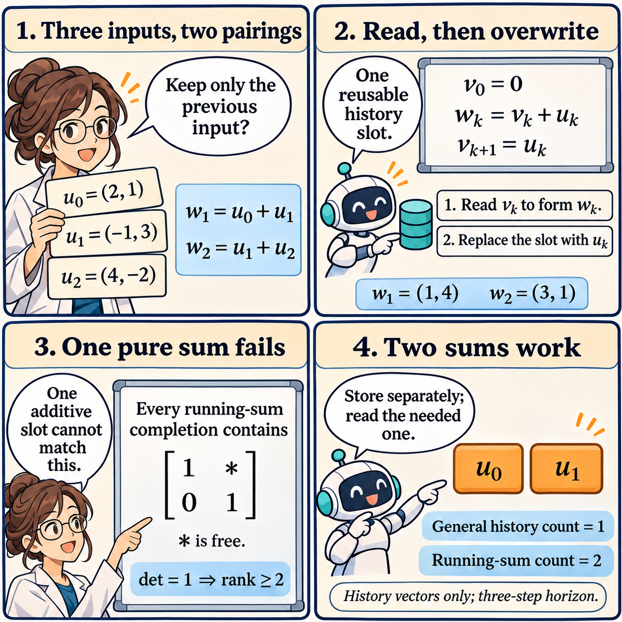
The directions are outputs of the linear update rule, rather than model iterates. The two-dimensional numbers illustrate an identity required for arbitrary inputs. Only history vectors enter the displayed storage counts.
This gap can grow with the horizon. For \(N\ge2\), ask at every step for the current input plus the previous one, with zero history initially. One reusable slot still suffices. In any running-sum completion, rows \(1,\ldots,N-1\) and columns \(0,\ldots,N-2\) form an upper-triangular block with diagonal entries one: entries below that block’s diagonal are prescribed zeros. Its determinant is one, so its rank is \(N-1\). The zero-filled subdiagonal shift attains that rank. Consequently, this family needs exactly \(N-1\) pure running sums and one general history vector.
There is also a delicate small-parameter limit. For \(\varepsilon\ne0\), the original three-step family has a one-running-sum implementation:
\[b_0=1,\quad b_1=1/\varepsilon,\quad c_1=1,\quad c_2=\varepsilon.\]After two inputs, that sum is \(u_0+u_1/\varepsilon\); reading it with weight \(\varepsilon\) produces \(\varepsilon u_0+u_1\). Thus its exact running-sum count is one for every nonzero \(\varepsilon\), but two at zero. This discontinuity has a scaling signature. Any rank-one completion must satisfy
\[\det\begin{pmatrix}1&z\\\varepsilon&1\end{pmatrix} =1-\varepsilon z=0, \qquad z=1/\varepsilon.\]That free completion entry diverges as \(\varepsilon\to0\). At \(\varepsilon=1/1024\), the inputs above produce the state \((-1022,3073)\) after two additions. Multiplication by \(1/1024\) recovers \((-511/512,3073/1024)\); adding \(u_2\) gives \(w_2=(1537/512,1025/1024)\). The reusable-state implementation reaches the same direction with bounded recurrence coefficients. Large internal values alone do not prove a rounding failure, but this example explains why minimizing the exact number of sums and finding a well-scaled realization are different design tasks.
Storage equivalence also needs a separate convergence argument. Continue the reset rule on the scalar objective \(f(x)=x^2/2\) with positive step size \(\eta\):
\[x_{k+1}=x_k-\eta(x_k+v_k),\qquad v_{k+1}=x_k.\]For \(k\ge1\), this becomes \(x_{k+1}=(1-\eta)x_k-\eta x_{k-1}\). Starting from \(x_0=1,v_0=0\), the choice \(\eta=1\) cycles through \(1,0,-1,0,1,\ldots\). The characteristic polynomial is
\[\lambda^2-(1-\eta)\lambda+\eta.\]For positive \(\eta\) its roots both lie strictly inside the unit circle exactly when \(\eta<1\). If the roots are nonreal, their modulus is \(\sqrt\eta\). If they are real and \(0<\eta<1\), their positive sum and product make both roots positive, and the larger root is below one since \(\sqrt{(1-\eta)^2-4\eta}<1+\eta\). For \(\eta\ge1\), their product rules out strict stability. At \(\eta=1/2\) the modulus is \(1/\sqrt2\), and the first iterates are \(1,1/2,-1/4,-3/8,-1/16,\ldots\). The same one-vector storage pattern therefore supports both a convergent recurrence and a cycle.
My research judgment is that optimizer storage should be measured together with the allowed state transitions and the conditioning of the realization. For large models, the distinction concerns full parameter-sized vectors, so a reset or restart can have a substantial storage consequence. The exact lower bounds above belong to the specified fixed-coefficient linear representation. They do not count activation memory or communication, and they do not establish a learning advantage.
A concrete next experiment would compare direct state recurrences and reconstructed running sums for the same coefficients while sweeping small transition factors and reset schedules. Measure state magnitudes and trajectory error alongside stored-vector counts. The paper’s reconstruction guarantees bound coefficient approximation, which is a useful starting point; sensitivity of the resulting optimization trajectory remains a separate question. The worked family makes that distinction visible before a large training system obscures it.
The comic was created with AI.