Training a sampler on its own outputs makes the distribution of its training data part of the algorithm. A plausible-looking collection of samples can have the wrong relative frequencies. Importance weights can change those frequencies, yet a correct weight formula and an accurate finite training population are different achievements.
Nguyen, Dau and Thiéry’s Amortizing Tempered Sampling with Corrected Self-Training, first public on November 17, trains a shared temperature-conditioned sampler using corrected populations and replay buffers. Proposals are weighted, resampled and moved by MCMC before a temperature bridge supplies the next buffer (Section 2). SSS, its diffusion implementation, computes discrete path weights without requiring the endpoint density (Section 3.2).
Write the tempered target as \(\pi_\beta(x)\propto\rho(x)e^{-\beta E(x)}\), with normalized reference \(\rho\), relative energy \(E\) and \(0\le\beta\le1\). The bridge factor \(e^{-(\beta'-\beta)E(x)}\) changes the target temperature; proposal-correction weights address a different mismatch.
The path construction can be understood directly. At fixed \(\theta\), let \(G\) be a reference Markov transition preserving \(\rho\). For a length-\(L\) proposal path, define
\[P_\theta(y_{0:L})=\rho(y_0)\prod_{n=0}^{L-1}Q_{\theta,n}(y_{n+1}\mid y_n), \qquad R_\beta(y_{0:L})=\rho(y_0)\prod_{n=0}^{L-1}G(y_{n+1}\mid y_n)e^{-\beta E(y_L)}.\]Use sums for discrete states or integrals for densities. Assume the proposal covers the extended target and the weighted test function is integrable. Since the reference chain ends with distribution \(\rho\), cancellation of path densities gives
\[w=R_\beta/P_\theta,\qquad \mathbb E_{P_\theta}[w f(Y_L)] =Z_\beta\,\mathbb E_{\pi_\beta}[f].\]Here \(Z_\beta\) is the target normalizing constant. This is an unnormalized expectation identity. Taking a random ratio of two sample averages introduces a further statistical question. The paper’s construction uses Gaussian Ornstein–Uhlenbeck transitions for \(G\); our finite example below isolates the weighting mechanism.
Consider two states, \(A\) and \(B\), with target and proposal probabilities
\[\pi=(1/4,3/4),\qquad q=(3/4,1/4),\qquad w(A)=\frac13,\quad w(B)=3.\]This is also a one-step instance of the path identity. Take uniform \(\rho\), let \(G\) independently draw from \(\rho\), choose \(e^{-E(A)}=1/2\) and \(e^{-E(B)}=3/2\), and let the proposal transition independently draw from \(q\). At \(\beta=1\), \(Z_1=1\) and the initial-state factor cancels, leaving exactly \(w(x)=\pi(x)/q(x)\). These categorical calculations isolate the correction mechanism.
Suppose a particular batch contains three \(A\) samples and one \(B\) sample. Its raw fraction of \(B\) is \(1/4\). The weighted masses are
\[W_A=3\left(\frac13\right)=1,\qquad W_B=1(3)=3,\qquad \widehat\pi(B)=\frac{W_B}{W_A+W_B}=\frac34.\]For this batch the corrected measure matches the target. If four points are resampled independently from that weighted batch, the number of resulting \(B\) points is nevertheless random: it is binomial with parameters \(4\) and \(3/4\). Even here, resampling gives the target fraction in expectation, rather than guaranteeing exactly three \(B\) points. This independent-resampling illustration is separate from the paper’s systematic resampling.
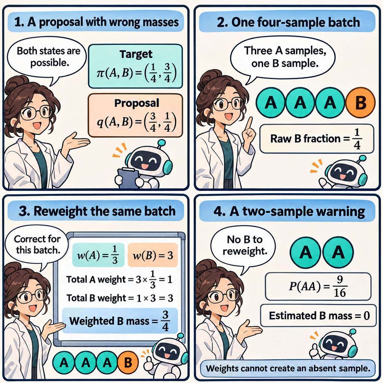
Panels 2–3 use one specified four-sample batch. Panel 4 switches to a two-sample batch to show a coverage failure. The weights act on the empirical measure before resampling.
Now draw only two independent proposal samples. The self-normalized estimate of \(\pi(B)\) is zero for \(AA\), \(9/10\) for either ordering of the mixed pair, and one for \(BB\). Their probabilities are \(9/16\), \(6/16\) and \(1/16\). Therefore
\[\mathbb E[\widehat\pi_2(B)] =\frac9{16}(0)+\frac6{16}\left(\frac9{10}\right)+\frac1{16}(1) =\frac25,\]although \(\pi(B)=3/4\). All probabilities and weights here are exact rational numbers, and both states have positive proposal probability. For comparison, the ordinary average \(\tfrac12\sum_i w(X_i)\mathbf1_{\{X_i=B\}}\) is unbiased for \(3/4\) here because the toy target is normalized. It can exceed one in an individual batch. Unbiasedness alone does not decide which estimator has smaller mean squared error.
The bias has a clean explanation for every finite batch size. If \(M\) is the number of \(B\) samples in \(N\) independent draws, then \(M\sim\operatorname{Binomial}(N,1/4)\) and
\[\widehat\pi_N(B)=h(M/N),\qquad h(r)=\frac{9r}{1+8r},\qquad h''(r)=-\frac{144}{(1+8r)^3}<0.\]Strict concavity gives \(\mathbb E[h(M/N)]<h(1/4)=3/4\) for every finite \(N\). The law of large numbers still gives convergence to \(3/4\) as \(N\) grows. This particular direction of bias follows from this binary family; it is not a general sign rule for importance sampling.
Coverage gives a second obstruction. The probability that an \(N\)-sample proposal batch contains no \(B\) is \((3/4)^N\). Achieving at least a 95% chance of seeing one \(B\) requires \(N\ge11\): the missing-state probabilities at \(N=10\) and \(N=11\) are approximately \(0.05631\) and \(0.04224\). Seeing one point is only a coverage requirement, not a guarantee of accurate mass estimation. On an all-\(A\) batch, changing weights or resampling cannot produce \(B\). MCMC can introduce new states, but target invariance alone does not promise mixing: the identity kernel preserves every distribution and leaves this batch unchanged.
Why does the training measure matter for a diffusion score? For a standard Gaussian reference, the paper’s score regression uses the label \(-\alpha\beta\nabla E(X)\), with \(X\) drawn from the target and \(X_t=\alpha X+\sqrt{1-\alpha^2}\xi\) for independent \(\xi\sim\mathcal N(0,I)\) (Section 3.1 and Appendix B). The population identity assumes differentiability, differentiation under the integrals, valid integration by parts and finite gradient second moments.
As a separate continuous example, set \(E(x)=3x^2/2\), \(\beta=1\) and \(\alpha=1/2\). The correct target is \(X\sim\mathcal N(0,1/4)\). Write \(Y=X/2+\sqrt{3/4}\xi\) for independent standard Gaussian \(\xi\). The regression label is \(-3X/2\). Gaussian conditioning gives
\[\mathbb E[X\mid Y=y] =\frac{\operatorname{Cov}(X,Y)}{\operatorname{Var}(Y)}y =\frac{1/8}{13/16}y=\frac2{13}y, \qquad r^*(y)=-\frac3{13}y.\]This agrees with the relative score of \(Y\sim\mathcal N(0,13/16)\): its score plus \(y\) is \(-16y/13+y=-3y/13\).
If an incorrect training buffer instead supplies \(X\sim\mathcal N(0,1)\), while the same energy label and perturbation rule are retained, then \(\operatorname{Cov}(X,Y)=1/2\) and \(\operatorname{Var}(Y)=1\). The population least-squares predictor becomes \(-3y/4\). Changing only the distribution of clean training points has changed the learned function. More optimization of this incorrect population objective preserves that discrepancy. Exact population reweighting restores the intended measure; a finite weighted buffer brings back the coverage and ratio-estimation issues above.
My research judgment is that corrected self-training should be evaluated as a coupled proposal-and-data system. Inspect mode masses and missing-mode frequency as well as weighted accuracy. Report the cost and quality of fresh raw proposals, newly corrected proposals and retained buffer draws separately. A stored population can be useful for repeated training while still limiting the distinct configurations available at evaluation.
The paper explicitly treats finite adaptive buffers as approximations and makes no fixed-buffer convergence claim for the self-training loop (Appendix A.2). A concrete next experiment would hold the proposal family and compute budget fixed while varying batch size, buffer capacity and inter-mode mobility of the rejuvenation kernel. Independent repeats should measure both the average estimated mode mass and the frequency of losing a mode. The binary calculation predicts persistent small-batch bias even with perfect weights; the Gaussian calculation shows how an incorrect training measure can then alter the learned score.
The comic was created with AI.